How to Use Conditional Formatting Based on VLOOKUP in Excel

In this article, you learn how to apply Conditional Formatting based on the VLOOKUP function with 3 different criteria in Excel.

Download Practice Template

You can download the free practice Excel template from here.

3 Criteria on Using Conditional Formatting Based on VLOOKUP in Excel

This section will help you to learn how to use Excel’s Conditional Formatting command to format your Excel worksheet in the condition that you require based on the VLOOKUP function.

1. Conditional Formatting to Compare Results Based on VLOOKUP in Excel

In this phase, we will learn how to compare results between two sheets based on VLOOKUP with Conditional Formatting in Excel.

As shown in the picture below, we have a dataset of students’ Names and Semester results in the Semester sheet.

In another sheet named Retake, we have a dataset of students’ Names and Retake results.

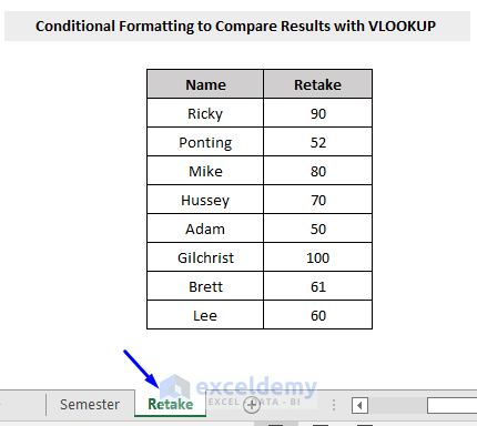
Now we will compare these two sheets and find out which student scored less in the semester exam that they had to take the retake exam with the help of Conditional Formatting and the VLOOKUP function.

Steps to do that are,

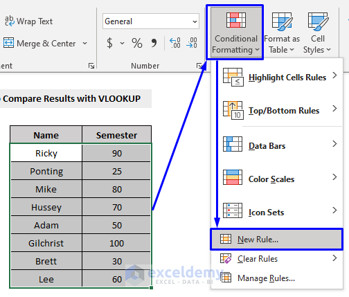
• Select the cells that you want to format (e.g. all the cells except headers from the Semester sheet).
• Then in the Home tab, select Conditional Formatting -> New Rule

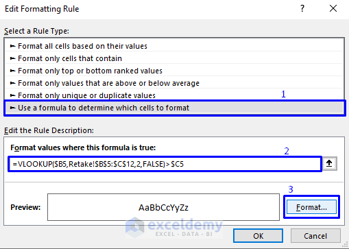
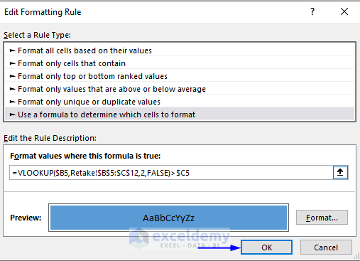
• In the Edit Formatting Rule pop-up window, select Use a formula to determine which cells to format as Rule Type and in the Edit the Rule Description box write the following formula,

Here,

$B5 = cell reference number of the first cell in the Semester sheet
Retake! = 2nd sheet to compare
$B$5:$C$12 = cell range to look up the value
2 = corresponding column number to extract the value from
FALSE = to get the exact match
$C5 = to compare the value with

• Next click Format.

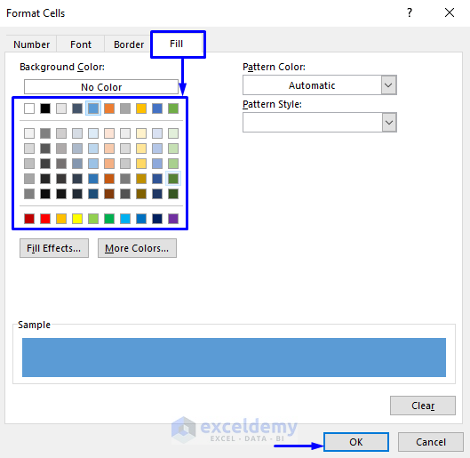
• Go to the Fill tab in the Format Cell window and pick any colour that you like.
• Click OK.

• Again click OK on the Edit Formatting Rule

The result is shown in the picture below.

In our dataset, only “Ponting” and “Brett” had scored relatively low so the result is highlighting their names and results.

Read more: How to Compare Two Columns in Excel For Finding Differences

2. Conditional Formatting to Match Results Based on VLOOKUP in Excel

In this part, we will see how to match results among two sheets in Excel using Conditional Formatting based on VLOOKUP.

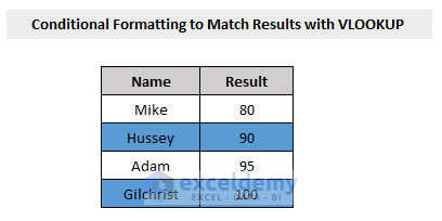
Look at the following picture where we have data of some student toppers from different departments in the Topper sheet.

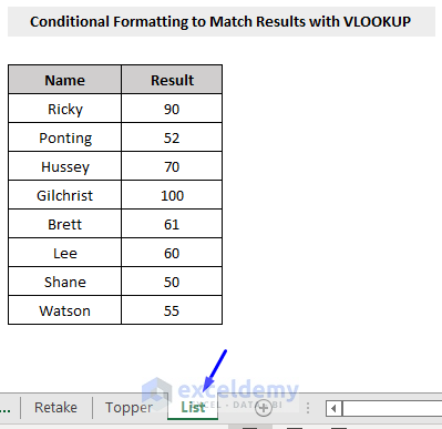
And in another sheet named List, we have a list of students’ names from one department.

So now we will see how to highlight only the data of the student toppers from the only department list that we have.

Steps to do that are,

• As shown in the previous phase, select the cells that you want to format (e.g. all the cells except headers from the Topper sheet) and in the Home tab, select Conditional Formatting -> New Rule.
• In the Edit Formatting Rule pop-up window, select Use a formula to determine which cells to format as Rule Type and in the Edit the Rule Description box write the following formula,

Here,

$B5 = cell reference number of the first cell in the Topper sheet
List! = 2nd sheet to compare
$B$5:$C$12 = cell range to look up the value
1 = corresponding column number to extract the value from
FALSE = to get the exact match
The ISNA function is to check whether the value is #N/A or not. If it is then it will return TRUE, otherwise FALSE.

• Next, similar to before, click Format, pick a colour from the Fill tab, click OK and OK.

The result is shown below.

Only the names “Hussey” and “Gilchrist” were in the List sheet in our workbook so those two names are highlighted in the Topper sheet.

Read more: How to Compare Two Columns Using Conditional Formatting in Excel

3. Conditional Formatting for Multiple Conditions for the Same Range Based on VLOOKUP in Excel

We can also utilize Conditional Formatting for multiple conditions with the VLOOKUP function in Excel.

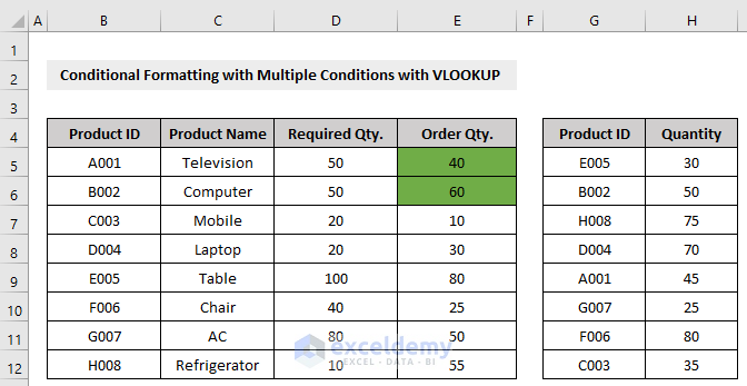
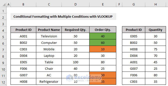
Consider the following data. We will format the Order Qty. into three categories based on the Quantity predefined by the seller.

Steps to do that are,

• As shown in the previous phase, select the cells that you want to format (e.g. all the cells except header in the Order Qty. column) and in the Home tab, select Conditional Formatting -> New Rule
• In the Edit Formatting Rule pop-up window, select Use a formula to determine which cells to format as Rule Type and in the Edit the Rule Description box write the following formula,

Here,

E5 = cell reference number of the first cell in the Order Qty. column
$G$5:$H$12 = cell range to match the value
2 = corresponding column number to extract the value from
FALSE = to get the exact match
The ABS function is for returning the absolute value of a number without its mathematical sign (e.g. +/- signs).

• Next, similar to before, click Format, pick a colour from the Fill tab (we picked Green), click OK and OK.

The result is shown below.

• Repeat the steps from selecting the cells to writing the formula. This time write the formula as,

Here,

E5 = cell reference number of the first cell in the Order Qty. column
B5 = to match the Product ID
$G$5:$H$12 = cell range to match the value
2 = corresponding column number to extract the value from
FALSE = to get the exact match

• Click Format, pick a colour from the Fill tab (we picked Red this time), click OK and OK.

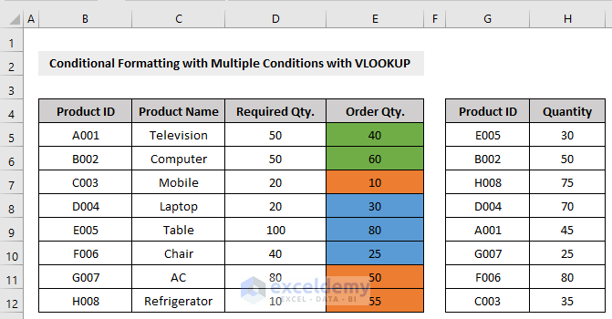
The result is shown below.

• Again repeat the steps from selecting the cells to writing the formula. And now write the formula as,

Here,

E5 = cell reference number of the first cell in the Order Qty. column
B5 = to match the Product ID
$G$5:$H$12 = cell range to match the value
2 = corresponding column number to extract the value from
FALSE = to get the exact match

• Click Format, pick a colour from the Fill tab (we picked Blue this time), click OK and OK.

The result is shown below.

Conclusion

This article showed you how to apply the Conditional Formatting command with the VLOOKUP function in Excel. I hope this article has been very beneficial to you. Feel free to ask any questions regarding the topic.

You May Also Like to Explore

• Conditional Formatting with INDEX-MATCH in Excel (4 Easy Formulas)
• Excel Conditional Formatting on Multiple Columns
• Conditional Formatting with Formula for Multiple Conditions in Excel
• How to Use Conditional Formatting in Excel [Ultimate Guide]