Method 1 – Using ISODD Function
Steps:
- Select the column where you want to change the text color.
- Go to the Home tab.
- Select the New Rule from the Conditional Formatting.
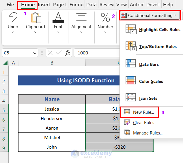
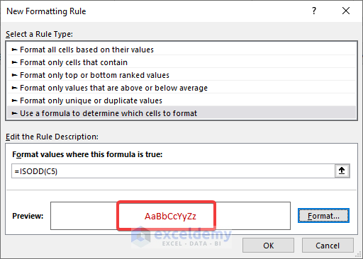
- Select Use a formula to determine which cells to format as the Rule Type.
- Write the formula as mentioned in the image. The formula is:
=ISODD(C5)- Click Format.

- Select the font color and press OK.
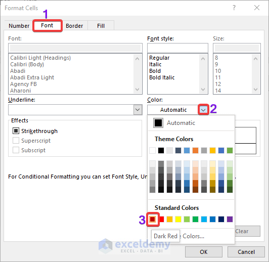
- Get a Preview of the font color.
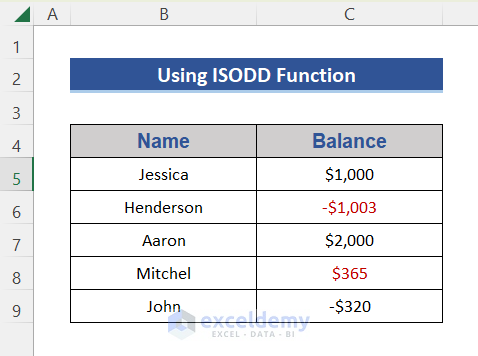
- Press OK, and we can see that the odd numbers on the Balance column are showing with changing color.
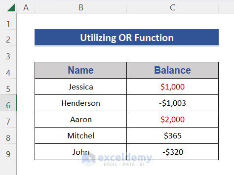
Method 2 – Changing Text Color Based on Value with OR Function
Steps:
- Select the desired column and go to the New Rule option, as shown previously.
- Write the formula:
=OR(B5="John",C5>400)- Select the format like previously.
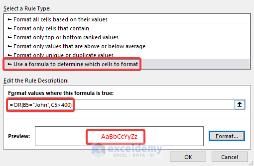
- Press OK and we see that the text color is changed.
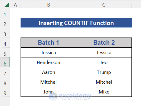
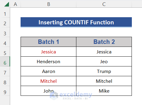
Method 3 – Applying COUNTIF Function to Change Text Color Based on Value
Steps:
- Modify the data set for applying the mentioned formula.
- Write the formula in the New Rule option shown previously.
- The formula will be:
=COUNTIF(C5,B5)>0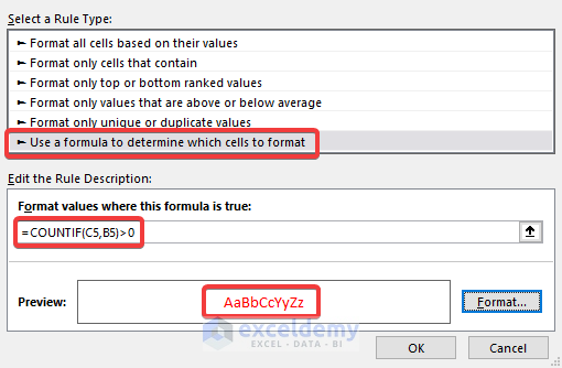
- Press OK and see that the matching names of column B are turned red as we mentioned.
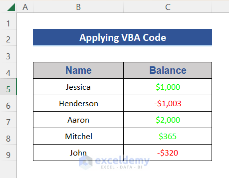
How to Apply VBA Code to Change Text Color Based on Value
Steps:
- Hold the Alt + F11 keys in Excel, which opens the Microsoft Visual Basic Applications window.
- Click the Insert button and select Module from the menu to create a module.

- Write the following code on the VBA command module.
Sub Text_Color()
Dim WorkRng As Range
xTitleId = "ExcelDemy"
Set WorkRng = Application.Selection
Set WorkRng = Application.InputBox("Range", xTitleId, WorkRng.Address, Type:=8)
For Each cell In WorkRng
If cell.Value > 0 Then
cell.Font.Color = vbGreen
ElseIf cell.Value < 0 Then
cell.Font.Color = vbRed
End If
Next
End Sub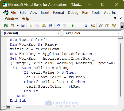
VBA Code Breakdown
- Create a new procedure Sub in the worksheet using the below statement.
Sub Text_Color()
- Declare variables as below.
Dim WorkRng As Range
xTitleId = "ExcelDemy"
- Set the variables and select the range.
Set WorkRng = Application.Selection
Set WorkRng = Application.InputBox("Range", xTitleId, WorkRng.Address, Type:=8)
- Activate it and start an IF loop for each cell. However, it checks the value and provides a preset color.
For Each cell In WorkRng
If cell.Value > 0 Then
cell.Font.Color = vbGreen
ElseIf cell.Value < 0
Then cell.Font.Color = vbRed
End If
Next
- End the Sub of the VBA macro as
End Sub- Press the F5 key to run the code.
- A dialog box will show the input range and we select a range.
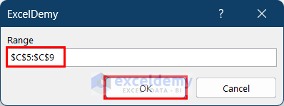
- Press OK and you will get your desired output.
Download Practice Workbook
Download this practice workbook to exercise while you are reading this article.
Related Articles
- How to Format Cell Based on Formula in Excel
- How to Use Conditional Formatting Based on VLOOKUP in Excel
- How to Apply Conditional Formatting with INDEX-MATCH in Excel
- Excel Conditional Formatting Formula with IF
- Excel Conditional Formatting Formula If Cell Contains Text
- Applying Conditional Formatting for Multiple Conditions in Excel
- Conditional Formatting If Cell is Not Blank
- Conditional Formatting Multiple Text Values in Excel
- Conditional Formatting Entire Column Based on Another Column in Excel
- Excel Highlight Cell If Value Greater Than Another Cell
<< Go Back to Conditional Formatting with Multiple Conditions | Conditional Formatting | Learn Excel
Get FREE Advanced Excel Exercises with Solutions!

I am a containment Engineer. I want a formula for Excel to return the words replace, review when the result cell shows “Fail”.I’d like the text to turn red as a visual aid.
I just cant get one to work.
I’m new to Excel.
Can you help me please.
Best regards
[email protected]
Dear COLYNN BURRELL,
Thanks for reading our article. Try the following formula to resolve your issue.
=IF(C5="Fail", TEXT("Replace, Review", "[$-409]@"), "")The formula indicates that if cell C5 contains text Fail, then the formula will return Replace, Review. If not, then the result it will return will be blank.
Formula Breakdown
● TEXT(“Replace, Review”, “[$-409]@”)
This formula returns Replace, Review each time.
● IF(C5=”Fail”, TEXT(“Replace, Review”, “[$-409]@”), “”)
This formula returns Replace, Review only for the text string Fail.
Now to add red color to the output, use the conditional formatting feature as illustrated in this article.
● Select the range D5:D9.
● Go through these steps: Home >> Conditional Formatting >> New Rule.
● Now, select Format only cells that contain from the Select a Rule Type section.
● Select Specific Text.
● Type Replace, Review.
● Click on Format.
● Select Font.
● Click on the arrow down icon in the color section.
● Select the color red.
● Click on OK.
● Click on OK again.
● And the output will be as follows as you have desired.
Note: However, you can’t change the color of the output just after applying the formula. You have to use conditional formatting for that.
If the problem still appears, kindly send us your Excel file and specify the exact problem you are facing.
Thank you
Best Wishes,
Raiyan Zaman Adrey