Change Font Color Based on Value of Another Cell in Excel

In this tutorial, we will demonstrate how to change font color based on the value of another cell. Here is an overview of the process.

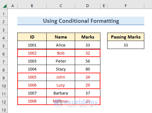
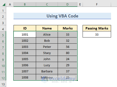
To demonstrate this tutorial, we’ll use this dataset:

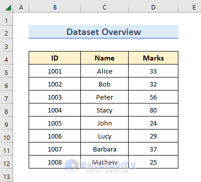
Our goal is to find the students who failed (scoring less than 33) and change the font color for those rows.

Method 1 – Using Conditional Formatting

Steps:

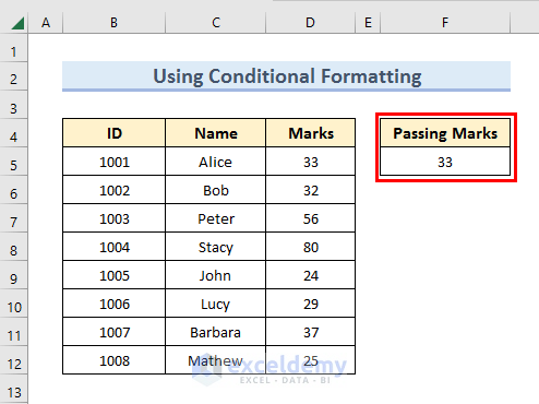
Add a criteria table like the image below.

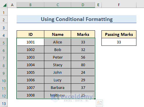
Select the range of cells B5:D12.

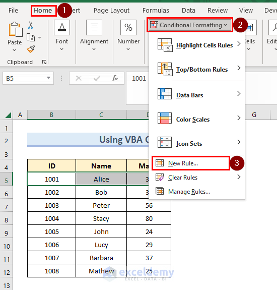
From the Home tab, select Conditional Formatting >> New Rule.

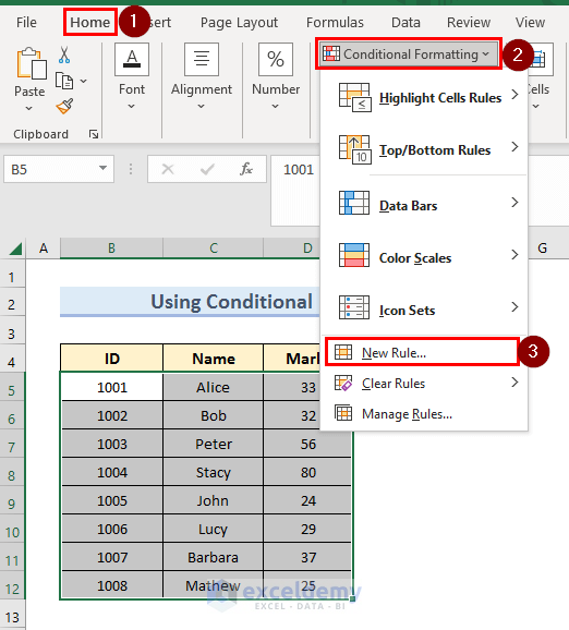
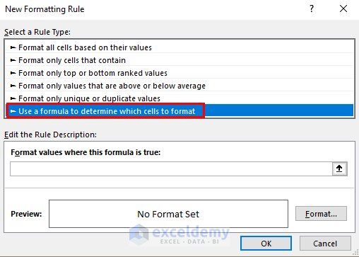
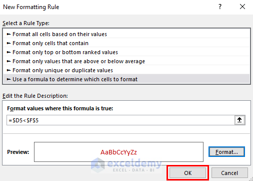
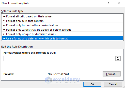
From the New Formatting Rule dialog box, select Use a formula to determine which cells to format.

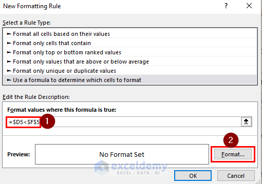
Enter the following formula in the field:

=$D5<$F$5

Click on Format.

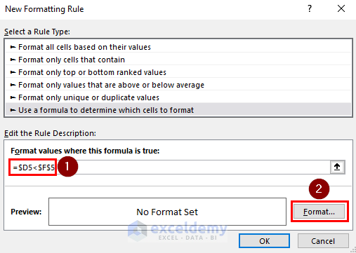
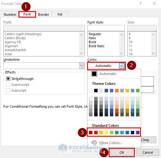
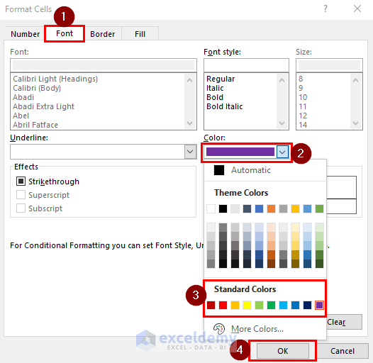
From the Format Cells dialog box, select the Font tab.
Choose any color from the dropdown menu.
Click on OK.

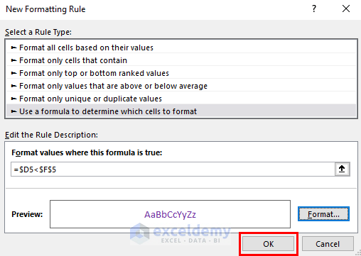
Click OK again.

The font color of the rows containing the students who failed changes to red.

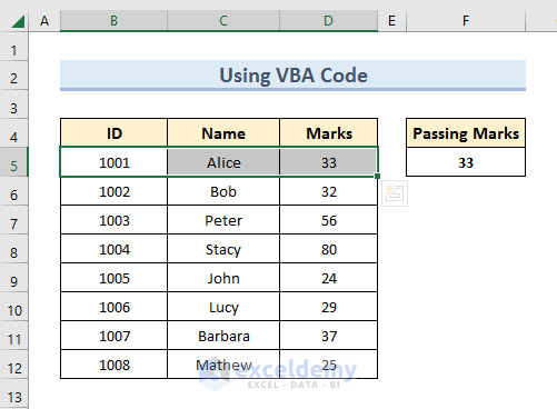
Method 2 – Using VBA Code

In this method, we’ll use conditional formatting on one row, then use a VBA macro to repeat across our dataset.

Steps:

Select the range of cells B5:D5.

From the Home tab, select Conditional Formatting > New Rule.

From the New Formatting Rule dialog box, select Use a formula to determine which cells to format.

Enter the following formula in the field:

=$D5<$F$5

Click on Format.

From the Format Cells dialog box select the Font option.
Choose any color from the dropdown menu.
Click on OK.

Click OK again.

The first row is formatted. Let’s copy it across all the rows.

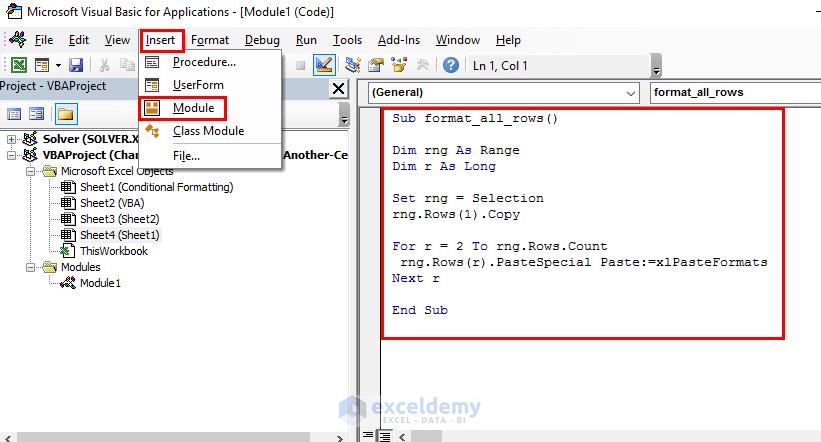
Press Alt+F11 on your keyboard to open the VBA Editor.
Click on Insert > Module.
Enter the following code in the module window:

Sub format_all_rows()
Dim rng As Range
Dim r As Long
Set rng = Selection
rng.Rows(1).Copy
For r = 2 To rng.Rows.Count
 rng.Rows(r).PasteSpecial Paste:=xlPasteFormats
Next r
End Sub

Save the file.

Select the range of cells B5:D12.

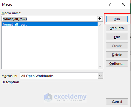
Press Alt+F8 to open the Macro dialog box.
Select the macro format_all_rows.
Click on Run.

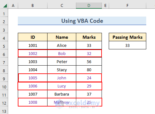
All the students with Marks less than 33 appear in color fonts.

Things to Remember

The VBA macro is just to copy the formats. It will individually create that formula for every row. If your dataset is large, this may take some time, but not as much as doing it manually!

Download the Practice Workbook

Change Font Color Based on Another Cell.xlsm