Method 1 – Simple Conditional Formatting Formula with IF in Excel
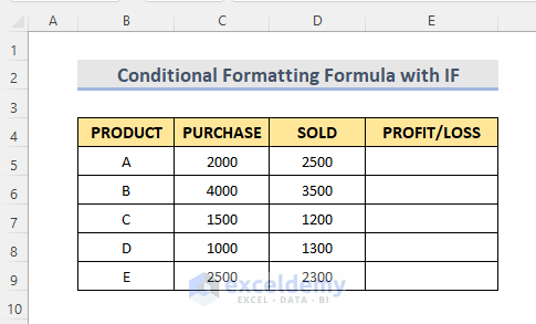
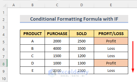
Consider a sample dataset of Products with their purchase and sold amounts. You can determine whether the products accrued a profit or loss in a single column with Conditional Formatting.
Steps:
- Select Cell E5.
- Type the formula:
=IF(D5>C5,"Profit","Loss")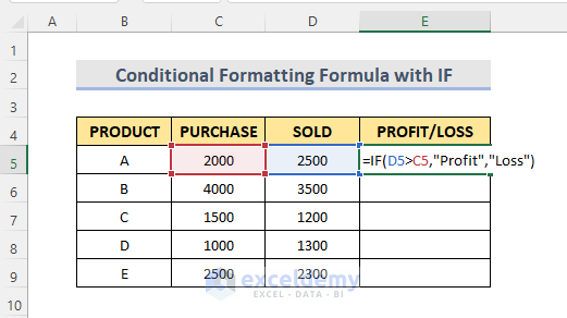
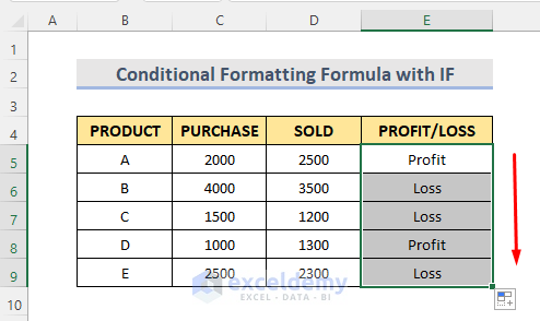
- Hit Enter and use the Fill Handle to autofill the next cells.
This will return “Profit” if cell D5 is greater than C5. Otherwise, it will return “Loss”.
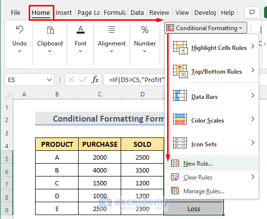
- Select the E column and go to the Home tab. From the Conditional Formatting drop-down, select New Rule.
- Click on the “Use a formula to determine which cells to format” option.
- In the formula box, type the formula:
=E5=”Profit”- Select the Format option.
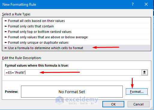
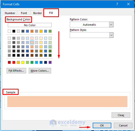
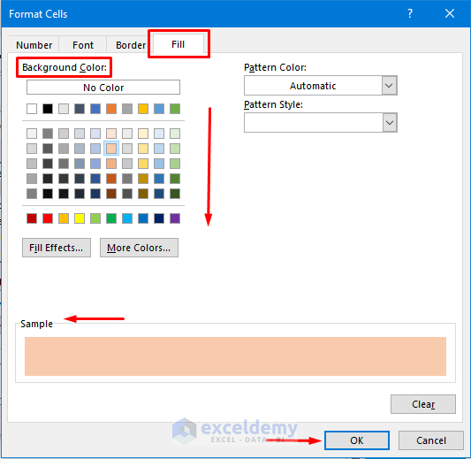
- In the Format Cells window, go to the Fill section.
- Choose any background color.
- Click on OK.
- Select OK again to exit the New Formatting Rule window.
- Note that the “Profit” cells are highlighted with color.
You can repeat the process for highlighting the “Loss” cells.
Read More: Excel Conditional Formatting Formula
Method 2 – Conditional Formatting Formula with Multiple IF Statements in Excel
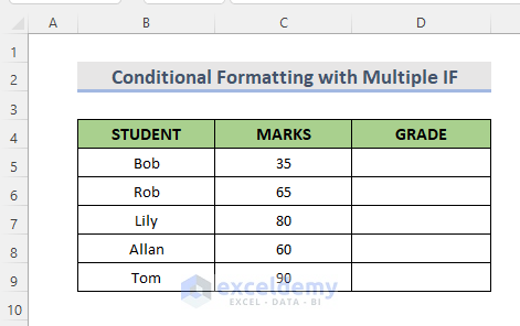
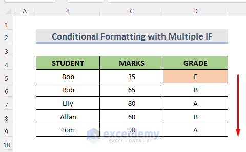
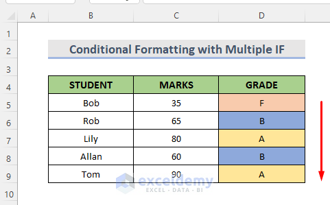
Consider a dataset (B4:D9) of student names and their marks. Let’s find the student’s grade and use conditional formatting to highlight the cells based on grade.
Steps:
- Select Cell D5.
- Input the formula:
=IF(C5<40,"F",IF(C5<70,"B","A"))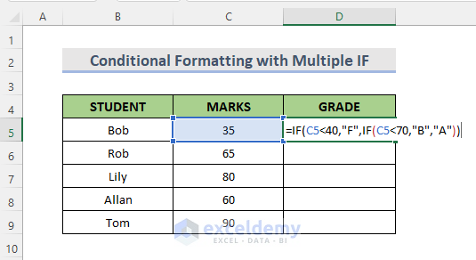
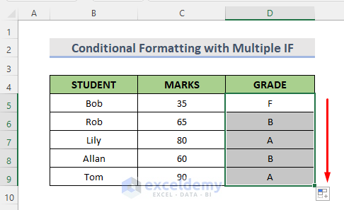
- Hit Enter and use the Fill Handle tool to apply the formula to other cells.
How Does the Formula Work?
IF(C5<70,”B”,”A”): This will return “B” if the marks are lower than 70. Otherwise, it returns “A”.
IF(C5<40,”F”,IF(C5<70,”B”,”A”)): This will return “F” if the mark is less than 40, or go to the next IF otherwise.
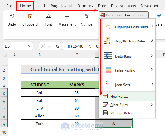
- Go to the Home tab > Conditional Formatting drop-down > New Rule.
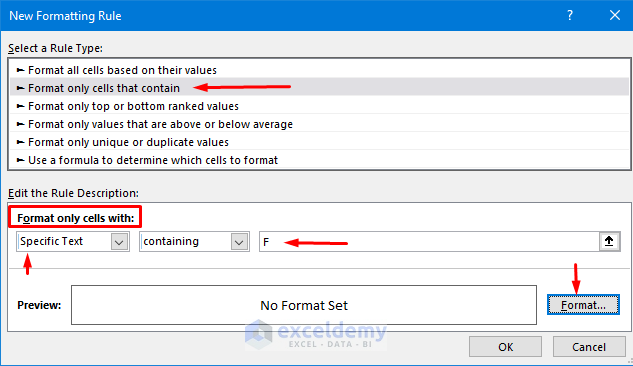
- In the New Formatting Rule window, select the “Format only cells that contain” option.
- Select Specific Text option from the drop-down of the Format only cells with box, then type “F” in the box on the right.
- Click on the Format option.
- In the Format Cells window, go to the Fill section and select the background color. You can preview the color sample in the Sample box.
- Select OK.
- Select OK again to close the Formatting Rule box.
- You can now see the cell containing “F” is colored.
- Repeat the process for Conditional Formatting with other grade texts and choose different colors.
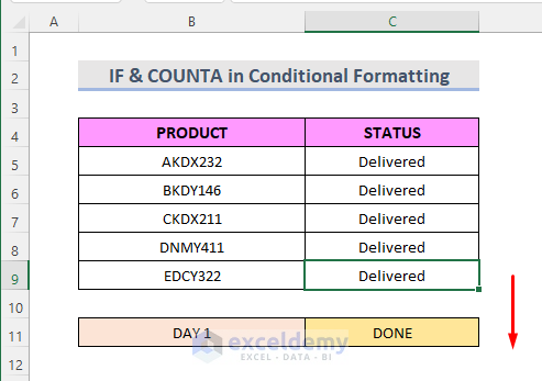
Method 3 – Using IF and COUNTA Functions in Excel Conditional Formatting
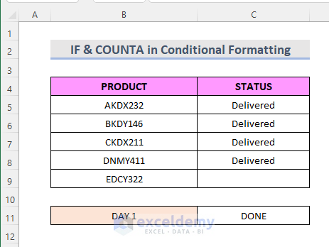
Here we have a dataset in which range B5:B9 contains product names and range C5:C9 contains their delivery status for Day 1. We are going to see that if the count of the “Delivered” in range C5:C9 is the same as the count of the products in range B5:B9, which will then format the cell C11 containing DONE to get a color.
Steps:
- Select cell C11 and go to the Home tab.
- Click on the Conditional Formatting drop-down.
- Choose New Rule.
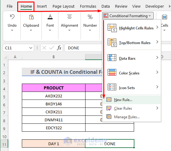
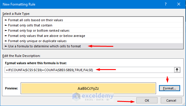
- Select the “Use a formula to determine which cells to format” option from the “New Formatting Rule” window.
- In the formula box, type the formula:
=IF(COUNTA($C$5:$C$9)=COUNTA($B$5:$B$9),TRUE,FALSE)- From the Format option, select a fill color like in the previous methods.
- Click on OK.
How Does the Formula Work?
- COUNTA($C$5:$C$9): Excel COUNTA function will count the number of cells in the C5:C9 range that contain values.
- COUNTA($B$5:$B$9): Excel COUNTA function will count the number of cells in the B5:B9 range that contain values.
- IF(COUNTA($C$5:$C$9)=COUNTA($B$5:$B$9),TRUE,FALSE): Excel IF function will return TRUE if the two ranges (B5:B9 & C5:C9) are equal, otherwise FALSE.
Results:
- When we type “Delivered” in cell C9, cell C11 gets colored.
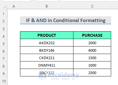
Method 4 – Combining IF and AND Functions to Apply Conditional Formatting in Excel
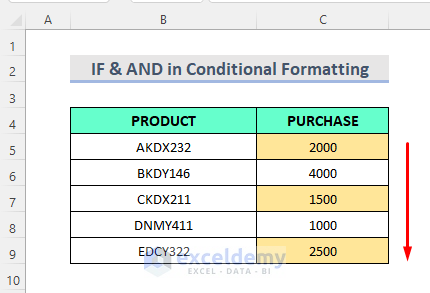
Consider a dataset (B4:C9) of products and their purchase amounts. Let’s color the products in the 1200-2800 purchase amount range.
Steps:
- Select the range of cells C5:C9 at first.
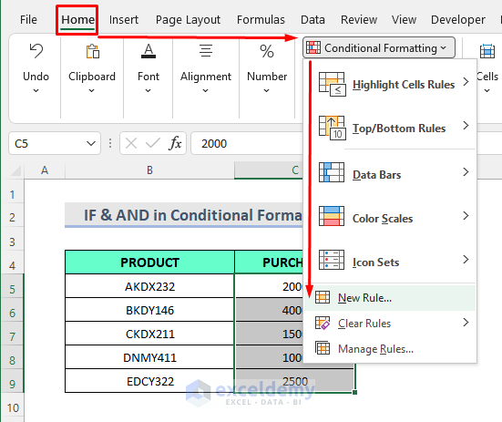
- Go to the Home tab.
- Select the Conditional Formatting drop-down.
- Click on the New Rule option.
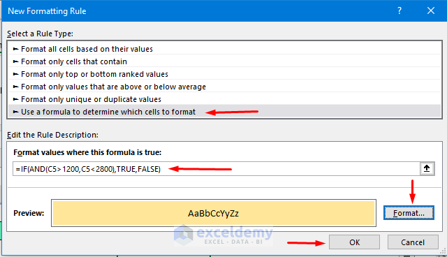
- From the New Formatting Rule window, select the “Use a formula to determine which cells to format” option.
- In the formula box, type the formula:
=IF(AND(C5>1200,C5<2800),TRUE,FALSE)- Select the specific color (see previous methods) from the Format option.
- Click on OK.
How Does the Formula Work?
- AND(C5>1200,C5<2800): This will return TRUE if cell C5 is greater than 1200 or less than 2800.
- IF(AND(C5>1200,C5<2800),TRUE,FALSE): This will return TRUE if cell C5 is in the 1200-2800 range, otherwise FALSE.
Results:
- Finally, we can see the cells are highlighted.
Download Practice Workbook
Download the following workbook and exercise.
Related Readings
- How to Format Cell Based on Formula in Excel
- How to Use Conditional Formatting Based on VLOOKUP in Excel
- How to Apply Conditional Formatting with INDEX-MATCH in Excel
- Excel Conditional Formatting Formula If Cell Contains Text
- Applying Conditional Formatting for Multiple Conditions in Excel
- Conditional Formatting If Cell is Not Blank
- How to Change Text Color Based on Value with Excel Formula
- Conditional Formatting Multiple Text Values in Excel
- Conditional Formatting Entire Column Based on Another Column in Excel
- Excel Highlight Cell If Value Greater Than Another Cell
<< Go Back to Conditional Formatting Formula | Conditional Formatting | Learn Excel
Get FREE Advanced Excel Exercises with Solutions!

I am trying to apply conditional formatting to a column of values that are generated from an equation. I don’t any cell with a formula to display a value unless it was calculated by the formula. So I use an equation to make that happen. The problem is, if I try to conditional format the cells to highlight based on whether or not the returned value is greater than zero, Excel highlights the sells that are not returning any values (blank cells) because Excel considers the equation itself as greater than zero. Any ideas on how to workaround this scenario?
Hi Jon,
You can try this path:
Select cell range > Click on Conditional Formatting > Select New Rules > Go to ‘Format only cells that contain’ option > From the Edit drop-down, select ‘No Blanks’ > Select Fill color > Press OK.