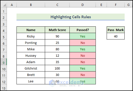
How to Make Yes Green and No Red in Excel

Example 1 – Highlighting Cells Rules

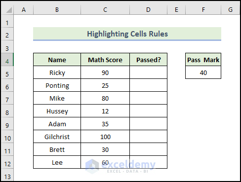
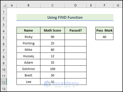
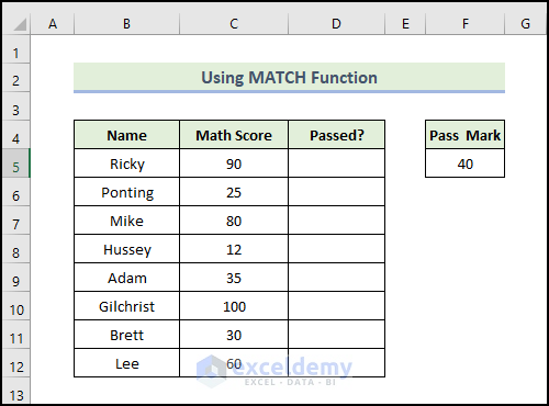
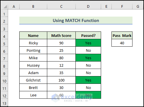
The dataset showcases students’ names and math scores.

Steps:

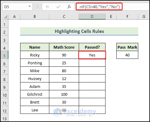
Enter the following formula in D5 to display pass and fail in the Passed column.

=IF(C5>40,"Yes","No")

The formula will check whether the value of C5 is greater than 40. If the condition is met, the function will return Yes. Otherwise, it returns No.

Press Enter.

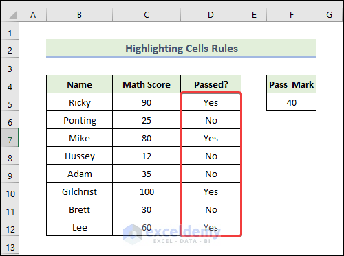
Drag the Fill Handle to fill the other cells.
This is the output.

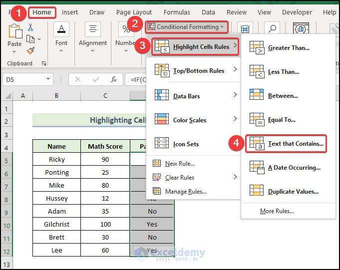
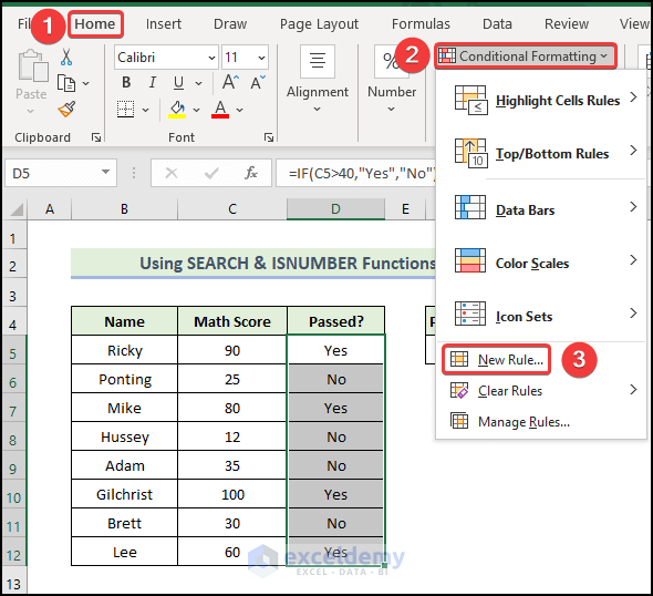
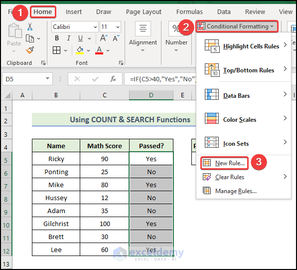
Select the cell range and go to the Home tab.
Select Conditional Formatting.
Choose Highlight Cells Rules.
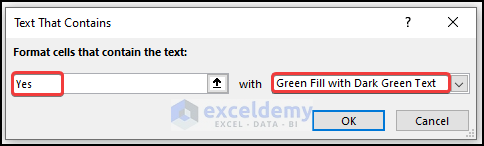
Select Text that Contains.

In the Text That Contains dialog box, enter Yes.
Choose a formatting style (here, Green File with Dark Green Text).
Click OK.

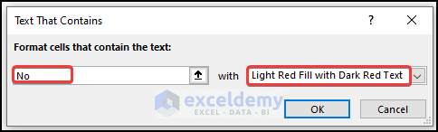
Repeat the above process
In the Text That Contains dialog box, enter No and select a formatting style (here, Light Red Fill with Dark Red Text).

Click OK.

This is the output.

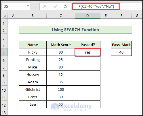
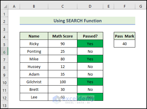
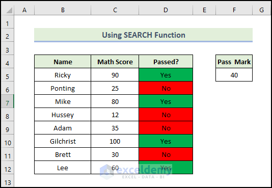
Method 2 – Using the SEARCH Function

Steps:

Use the following formula in D5 to display pass and fail in the Passed column.

=IF(C5>40,"Yes","No")

The formula checks whether the value of C5 is greater than 40. If the condition is met, the function will return Yes. Otherwise, it returns No.

Press Enter.

Drag the Fill Handle to fill the other cells.
This is the output.

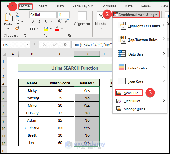
Select the range and go to the Home tab.
Choose Conditional Formatting.
Select New Rule.

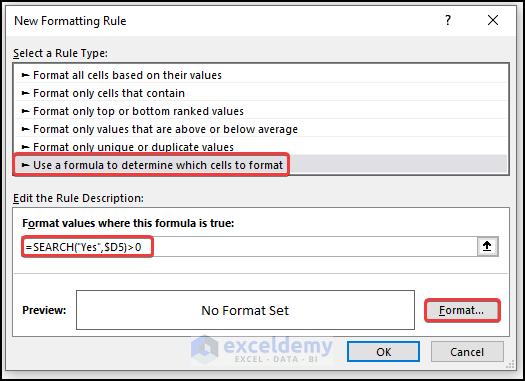
In the New Formatting Rule window, select Use a formula to determine which cells to format.
Enter the following formula in Format values where this formula is true.

=SEARCH("Yes",$D5)>0

The SEARCH function will look for Yes in the cells of column D and return a value for Yes.

Click Format.

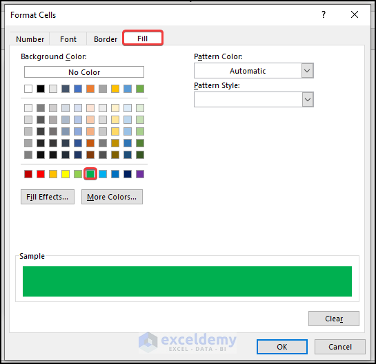
In the Format Cells dialog box, In Fill, choose Green as Background Color.
Click OK.

Click OK.

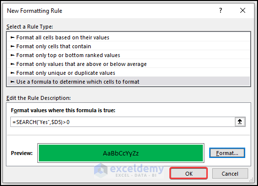
This is the output.

Follow the same procedure to see no in red.
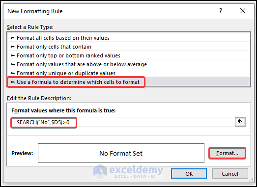
In the New Formatting Rule window, select Use a formula to determine which cells to format.
Enter the following formula in the Format values where this formula is true.

=SEARCH("No",$D5)>0

The SEARCH function will look for No in the cells of column D return a value.

Click Format.

In the Format Cells dialog box, select Fill.
Choose Red as Background Color, and click OK.

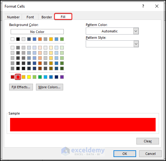
Click OK.

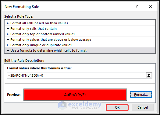
This is the output.

Method 3 – Applying the SEARCH and ISNUMBER Functions

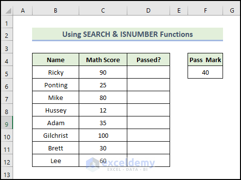
Steps:

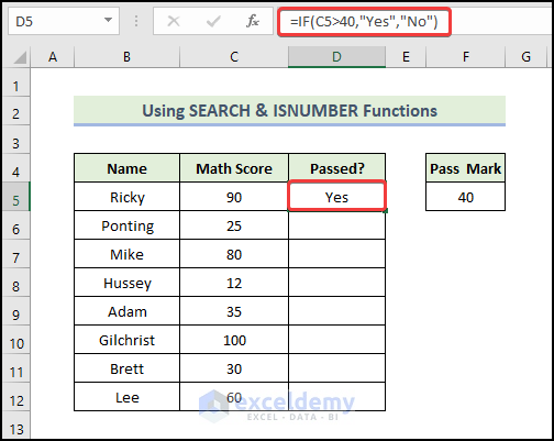
Use the following formula in D5..

=IF(C5>40,"Yes","No")

This formula will check whether the value of C5 is greater than 40. If the condition is met, the function will return Yes. Otherwise, it returns No.

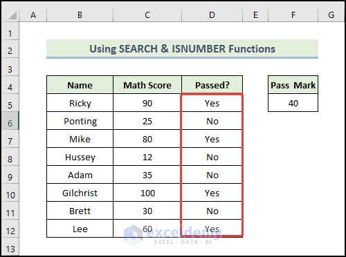
Press Enter.

Drag the Fill Handle to fill the other cells.

You will see the result in the Passed column.

Select the range.
Go to the Home tab and select Conditional Formatting.
Select New Rule.

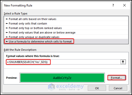
In the New Formatting Rule window, choose Use a formula to determine which cells to format.
Enter the following formula in Format values where this formula is true.

=ISNUMBER(SEARCH("Yes",$D5))

The SEARCH function will look for Yes in the cells of column D and return a value. The ISNUMBER will return TRUE if it gets a numeric value. Otherwise, FALSE.

Choose Green as Background Color in Format.
Click OK.

This is the output.

Follow the same procedure display no in red.
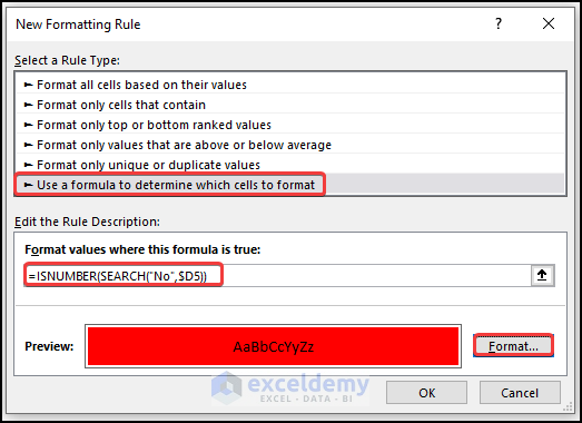
In New Formatting Rule, select Use a formula to determine which cells to format.
Enter the following formula in Format values where this formula is true.

=ISNUMBER(SEARCH("No",$D5))

The SEARCH function will look for No in the cells of column D and return a value. The ISNUMBER will return TRUE if it gets a numeric value. Otherwise, FALSE.

Choose Red as Background Color in Format.
Click OK.

This is the output.

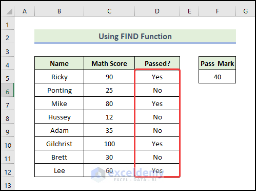
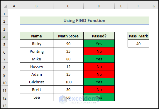
Method 4 – Using the FIND Function

Steps:

Use the following formula in D5.

=IF(C5>40,"Yes","No")

This formula will check whether the value of C5 is greater than 40. If the condition is met, the function will return Yes. Otherwise, it returns No.

Press Enter.

Drag the Fill Handle to fill the other cells.
This is the output.

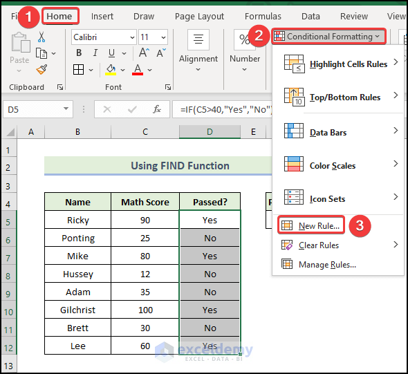
Select the range and go to the Home tab.
Choose Conditional Formatting.
Select New Rule.

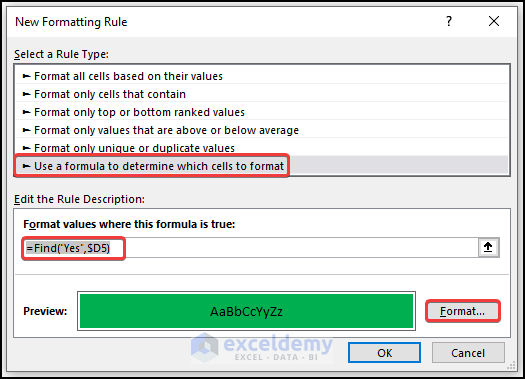
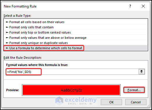
In the New Formatting Rule window, select Use a formula to determine which cells to format.
Enter the following formula in Format values where this formula is true.

=Find("Yes",$D5)

The FIND function will look for Yes in the cells of column D and, finding matches, will return Yes. No matches will not return any value.

Choose Green as Background Color in Format.
Click OK.

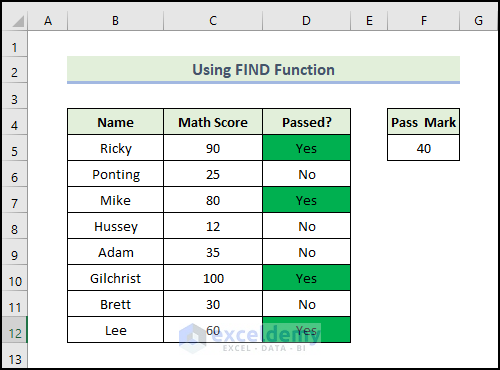
This is the output.

Follow the same procedure to display no in red
In New Formatting Rule, select Use a formula to determine which cells to format.
Enter the following formula in Format values where this formula is true.

=Find("No",$D5)

The FIND function will look for Yes in the cells of column D and, finding matches, will return Yes. Yes. No matches will not return any value.

Choose Red as Background Color in Format.
Click OK.

This is the output.

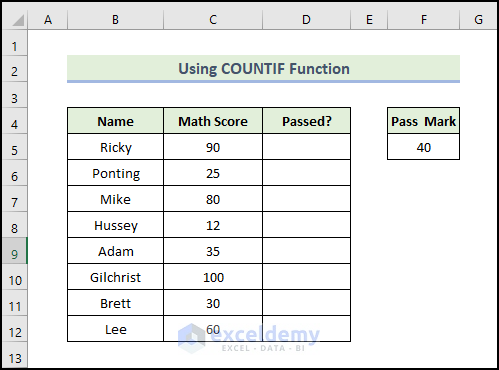
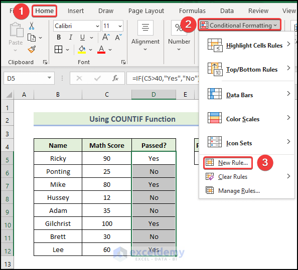
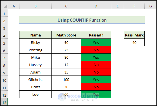
Method 5. Utilizing the COUNTIF Function

Steps:

Use the following formula in D5 to display pass and fail in the Passed column.

=IF(C5>40,"Yes","No")

The formula will check whether the value of C5 is greater than 40. If the condition is met, the function will return Yes. Otherwise, it returns No.

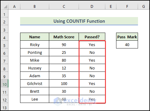
Press Enter.

Drag the Fill Handle to fill the other cells.
This is the output.

Select the range and go to the Home tab.
Choose Conditional Formatting.
Select New Rule.

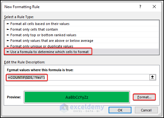
In the New Formatting Rule window, select Use a formula to determine which cells to format.
Enter the following formula in Format values where this formula is true.

=COUNTIF($D5,"*Yes*")

The wildcard symbol (*) before and after Yes returns partial matches and the COUNTIF function will return the number of times this text appears in column D.

Choose Green as Background Color in Format.
Click OK.

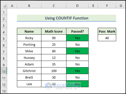
This is the output.

Follow the same procedure to display no in red
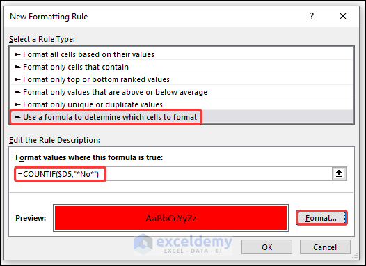
In New Formatting Rule, select Use a formula to determine which cells to format.
Enter the following formula in Format values where this formula is true.

=COUNTIF($D5,"*No*")

The wildcard symbol (*) before and after No returns partial matches and the COUNTIF function will return the number of times this text appears in column D.

Choose Red as Background Color in Format.
Click OK.

This is the output.

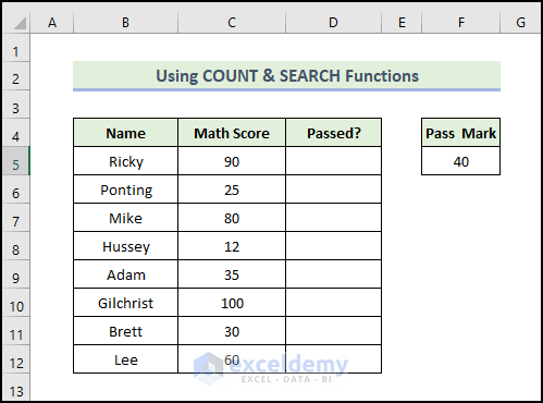
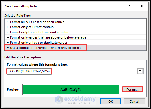
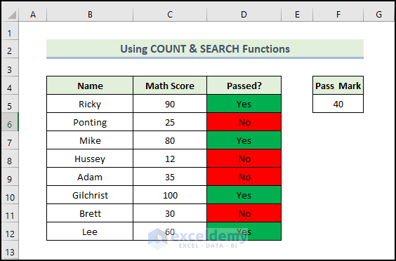
Method 6 – Combining the COUNT and SEARCH Functions

Steps:

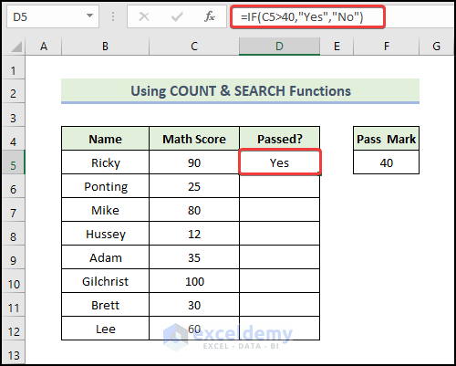
Use the following formula in D5 to display pass and fail in the Passed column.

=IF(C5>40,"Yes","No")

This formula will check whether the value of C5 is greater than 40. If the condition is met, the function will return Yes. Otherwise, it returns No.

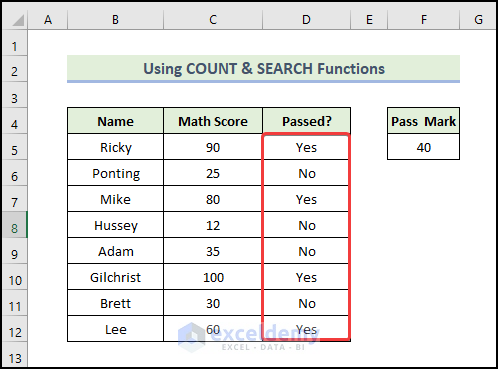
Press Enter.

Drag the Fill Handle to fill the other cells.
This is the output.

Select the range and go to the Home tab.
Choose Conditional Formatting.
Select New Rule.

In New Formatting Rule, select Use a formula to determine which cells to format.
Enter the following formula in Format values where this formula is true.

=COUNT(SEARCH("Yes",$D5))

The SEARCH function will look for Yes in column D and, finding matches, it will return a value. The COUNT function will return 1 if it gets any number from the output of the SEARCH function, otherwise 0.

Choose Green as Background Color In Format.
Click OK.

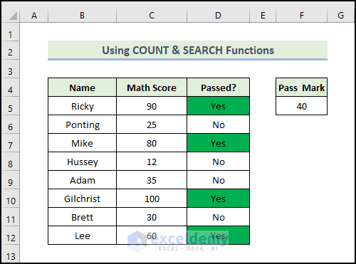
This is the output.

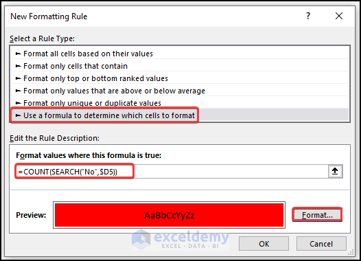
Follow the same procedure to display no in red
In New Formatting Rule, select Use a formula to determine which cells to format.
Enter the following formula in Format values where this formula is true.

=COUNT(SEARCH("No",$D5))

The SEARCH function will look for No in column D and, finding matches, will return a value. The COUNT function will return 1 if it gets any number from the output of the SEARCH function, otherwise 0.

Choose Red as Background Color in Format.
Click OK.

This is the output.

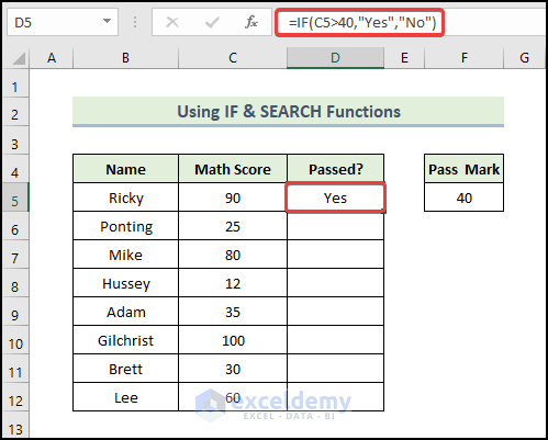
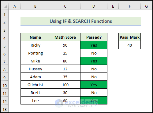
Method 7 – Applying the IF and the SEARCH Functions

Steps:

Use the following formula in D5 to display pass and fail in the Passed column.

=IF(C5>40,"Yes","No")

The formula will check whether the value of C5 is greater than 40. If the condition is met, the function will return Yes. Otherwise, it returns No.

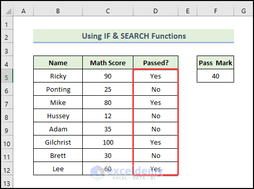
Press Enter.

Drag the Fill Handle to fill the other cells.

This is the output.

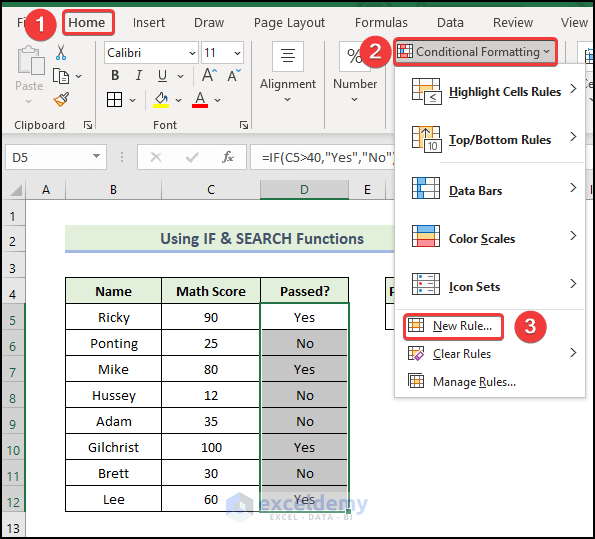
Select the range and go to the Home tab.
Choose Conditional Formatting.
Select New Rule.

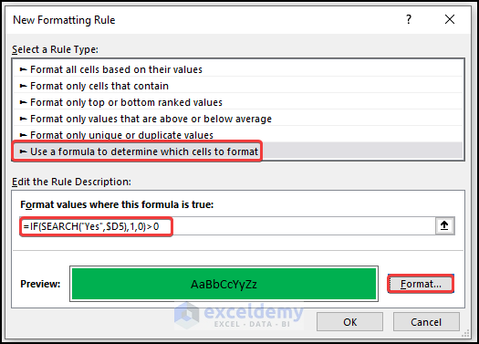
In New Formatting Rule, select Use a formula to determine which cells to format.
Enter the following formula in Format values where this formula is true.

=IF(SEARCH("Yes",$D5),1,0)>0

The SEARCH function will look for Yes in column D and, finding matches, will return a value. The IF will return 1 if the SEARCH function finds any matches, otherwise 0, and for values greater than 0, it will return TRUE. Otherwise, FALSE.

Next, choose Green as Background Color in Format.
Click OK.

This is the output.

Follow the same procedure to display no in red
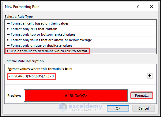
In New Formatting Rule, select Use a formula to determine which cells to format.
Enter the following formula in Format values where this formula is true.

=IF(SEARCH("No",$D5),1,0)>0

The SEARCH function will look for No in Column D and, finding matches, will return a value. The IF function will return 1 if the SEARCH function finds any matches, otherwise, 0.For values greater than 0, it will return TRUE, otherwise, FALSE.

Choose Red as Background Color in Format.
Click OK.

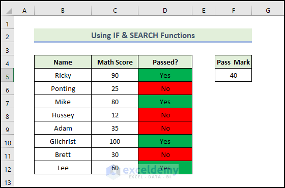
This is the output.

Method 8 – Utilizing the MATCH Function

Steps:

Use the following formula in D5 to display pass and fail in the Passed column.

=IF(C5>40,"Yes","No")

This formula will check whether the value of C5 is greater than 40. If the condition is met, the function will return Yes. Otherwise, it returns No.

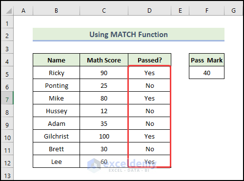
Press Enter.

Drag the Fill Handle to fill the other cells.

This is the output.

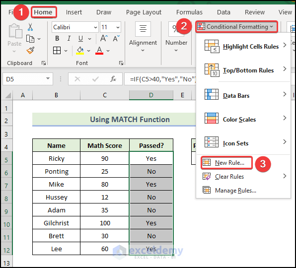
Select the range and go to the Home tab.
Choose Conditional Formatting.
Select New Rule.

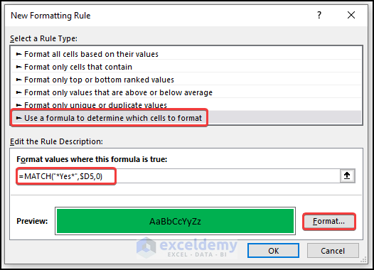
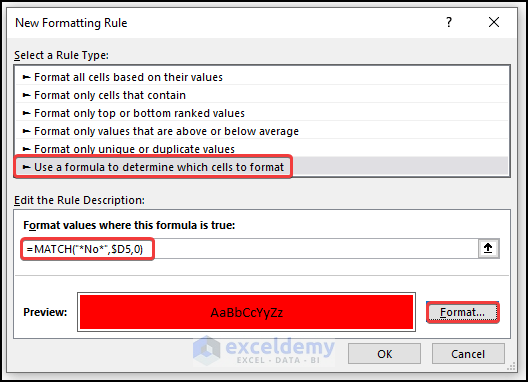
In New Formatting Rule, select Use a formula to determine which cells to format.
Enter the following formula in Format values where this formula is true.

=MATCH("*Yes*",$D5,0)

The wildcard symbol (*) before and after Yes, returns complete matches and the MATCH function will return 1, finding any partial matches in column D.

Next, choose Green as Background Color in Format.
Click OK.

This is the output.

Follow the same procedure to display no in red
In New Formatting Rule, select Use a formula to determine which cells to format.
Enter the following formula in Format values where this formula is true.

=MATCH("*No*",$D5,0)

The wildcard symbol (*), before and after No, returns complete matches and the MATCH function will return 1, finding partial matches in column D.