How to Copy Conditional Formatting with Relative Cell References in Excel – 2 Methods

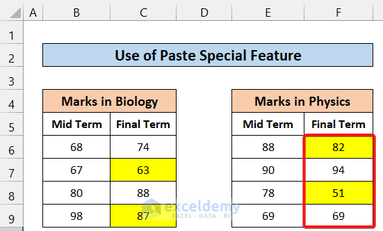
The sample dataset showcases 4 students’ marks at Midterm and Final Term in Biology and Physics.

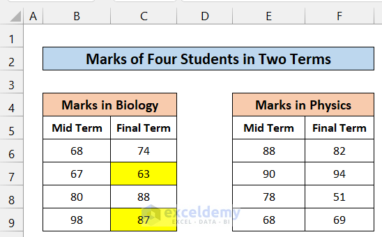
In Biology, the final term marks are lower than the Mid Term marks and were highlighted in yellow, using conditional formatting:

The conditional formula used in $C$6:$C$9 is =C6<B6. To copy the conditional formula and paste it into F6:F9:

Method 1 – Utilizing the Format Painter to Copy the Conditional Format with Relative Cell Reference in Excel

Steps:

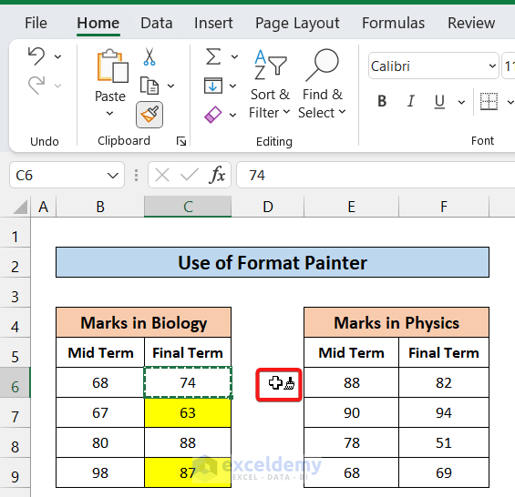
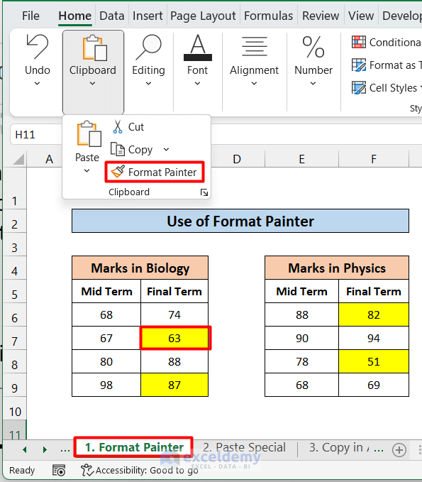
• Select a cell with the conditional formatting you want to copy. Here, C6.
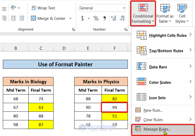
• In the Home tab, click Format painter in Clipboard.

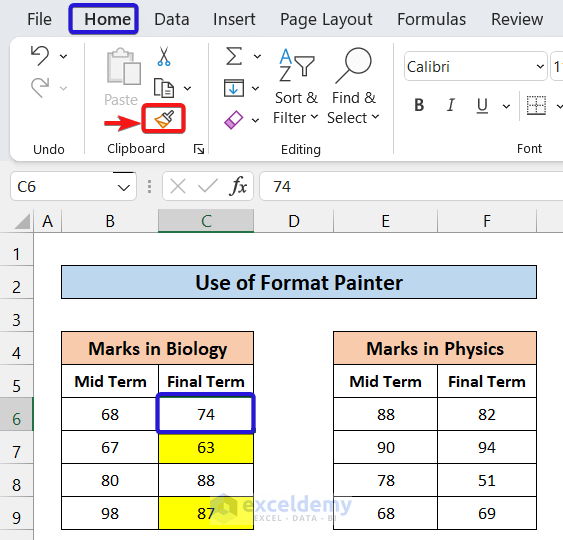
• A paintbrush icon is displayed.

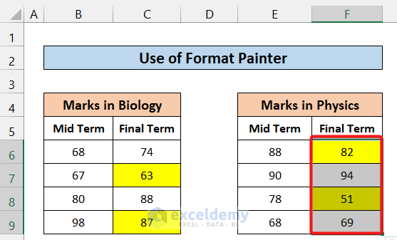
• Move the icon to F6, left-click and drag it to F9.

F6:F9 display conditional formatting.

• Observe the GIF below.

• To check the formula of the conditional formatting of a cell, click the cell and go to Conditional Formatting.
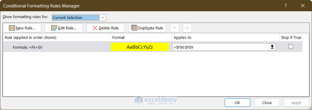
• Choose Manage Rules…

• Here, F7 displays: (F6<E6).

Read More: How to Copy Conditional Formatting to Another Cell in Excel

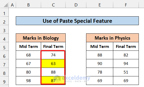
Method 2 – Copying Conditional Formatting with Relative Cell reference Using the Paste Special Feature in Excel

Steps:

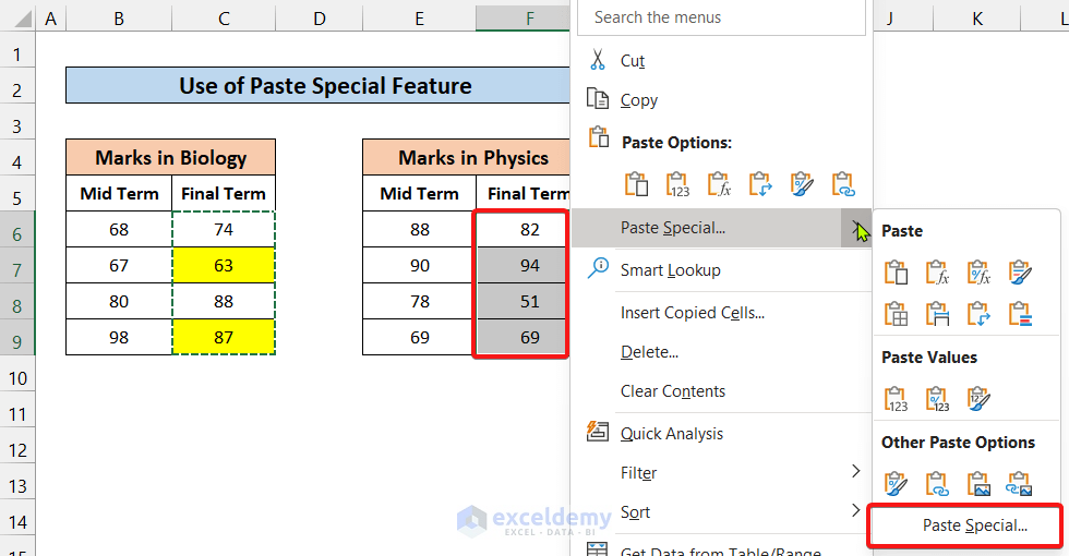
• Select the cells that contain conditional formatting. Here, C6:C9.

• Press Ctrl+C to copy.
• Select F6:F9 and right-click.
• Select Paste Special.

• Select Formats and click OK.

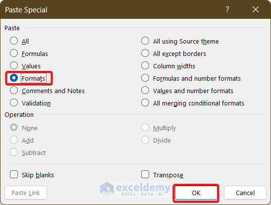
F6:F9 display conditional formatting.

• To check the formula of conditional formatting, follow the steps described described in Method 1.

Read More: How to Copy Conditional Formatting Color to Another Cell in Excel

How to Copy Conditional Formatting to Another Sheet in Excel

Steps:

• Click a cell containing conditional formatting. Here, C7, in 1. Format Painter sheet.
• Click Format Painter in Clipboard.

• Go to another sheet. Here, 3. Copy in Another Sheet.

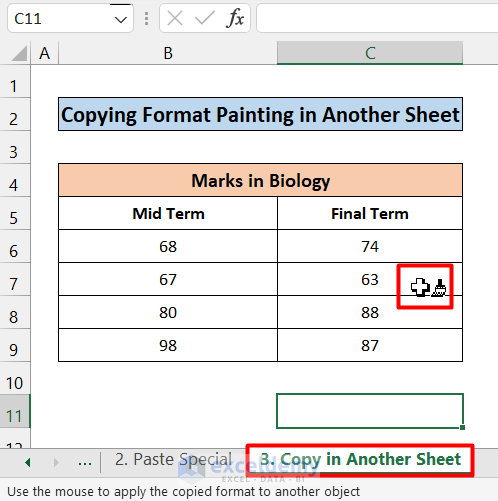
• Left-click the top cell (here, C6) to paste the format and drag down the Fill Handle.

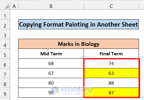
• Check the formula of the conditional formatting, as described above.

Download Practice Workbook

Download the practice workbook.

Related Articles

• How to Make Yes Green and No Red in Excel
• How to Create a Rating Scale in Excel
• How to Use Conditional Formatting on Text Box in Excel
• How to Apply Borders in Excel with Conditional Formatting
• How to Apply Alignment in Excel Conditional Formatting
• How to Copy Conditional Formatting to Another Sheet
• How to Copy Conditional Formatting to Another Workbook in Excel
  
• How to Copy Conditional Formatting But Change Reference Cell in Excel

<< Go Back to Copy Conditional Formatting | Conditional Formatting | Learn Excel