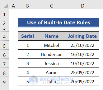
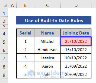
Example 1 – Using Built-In Date Rules
We’ll format the rows where the joining dates are within the past 7 days (Current date: 25-10-22).
Steps:
- We stored the name of employees and their joining dates in the dataset.
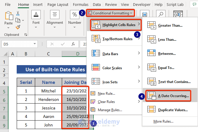
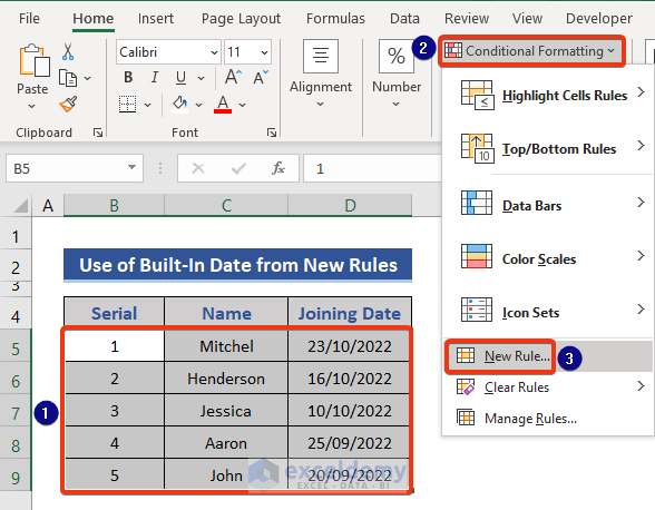
- Select the cells you want to apply the conditional formatting on (In our case, Range D5:D9).
- Go to Home and select the Conditional Formatting option under the Style section.
- Select the Highlight Cell Rules option and select the A Date Occurring option.
- A new window named A Date Occurring should appear.
- Select the In the last 7 days option from the first drop-down menu.
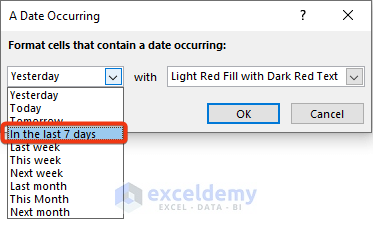
- Select the default color for highlighting cells.
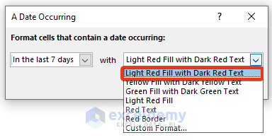
- Hit OK.
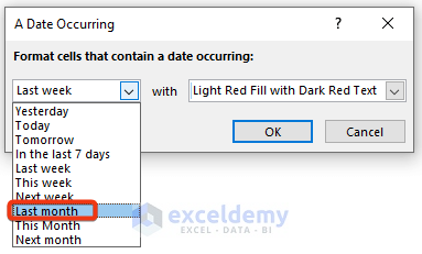
We want to highlight the dates of the last month.
- Go to the A Date Occurring window as shown previously.
- Choose the Last Month option from the drop-down list.
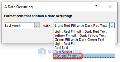
- Click on the drop-down symbol for the highlighting color.
- Choose the Custom Format option.
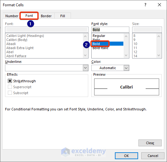
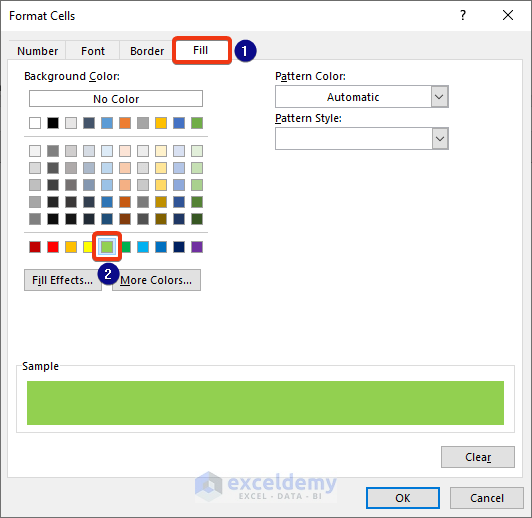
- The Format Cells window appears.
- Go to the Font tab.
- Choose Bold as the desired Font style.
- Move to the Fill tab.
- Choose the desired color from the list.
- Press the OK button.
- Here’s the result.
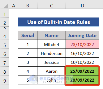
In short in this section, we get options for yesterday, today, tomorrow, last week, this week, next week, last month, this month, and next month. We can avail of those options without using any other formula or technique.
Alternative Method:
Steps:
- Click on the drop-down list of Conditional Formatting.
- Click on the New Rule option.
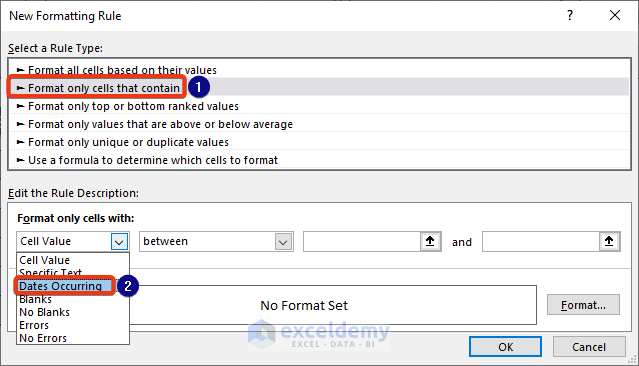
- The New Formatting Rule window appears.
- Select Format only cells that contain.
- Go to Edit the Rule Description section.
- Choose the Dates Occurring option from the list.
- You get a new drop-down field beside the previous section.
- Click on the down arrow.
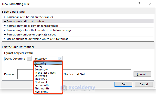
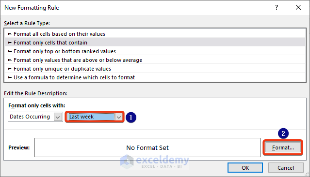
- Choose the Last week option.
- Click on the Format option.
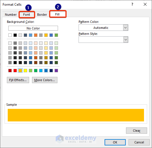
- Choose the desired Font and Fill color from the Format Cells window.
- Press the OK button.
- Go back to the previous window and see the Preview of the result.
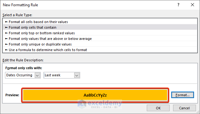
- Click on the OK button.
Read More: Conditional Formatting Based on Date in Another Cell in Excel
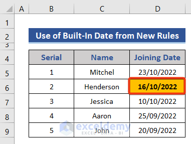
Example 2 – Highlight Dates Preceding the Current Date Using the NOW or TODAY Function
- Using the TODAY function – It returns the current date.
- Using the NOW function – It returns the current date with the current time.
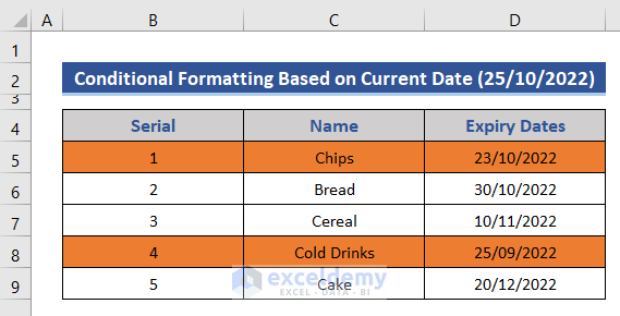
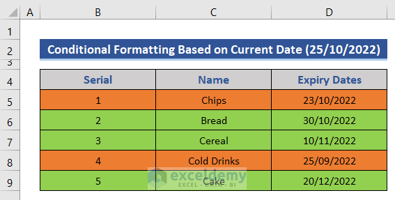
We want to format the cells and highlight the date expired products based on the current date (25/10/22). We’ll highlight the cells with two colors: one for the date expired products and another one for products within the expiry date.
Steps:
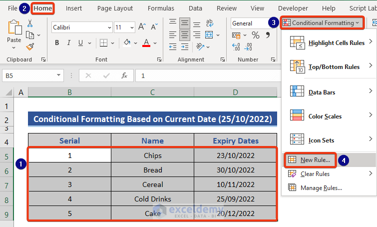
- Select the cells you want to apply the conditional formatting on (In our case, B5:D9).
- Go to Home and select the Conditional Formatting option under the Style section.
- Select the New Rule option from the drop-down menu.
- A new window named New Formatting Rule should appear.
- Select the Use a formula to determine which cells to format rule type.
- Enter the following formula in the specified field.
=$D5<NOW()
- Select the Format feature.
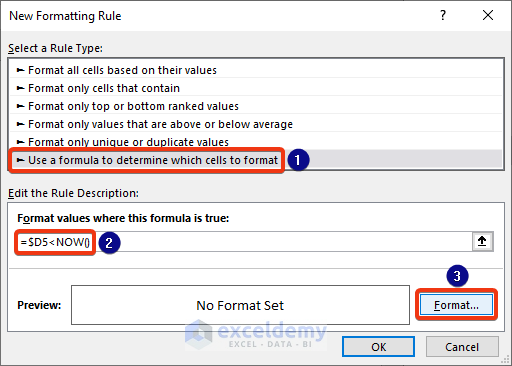
=$D5<NOW() checks whether the dates in Column D are less than the current date. If the date satisfies the conditions, then it formats the cell)
- Select the desired format (see Example 1) and click OK.
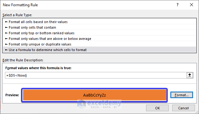
- Press the OK button.
We want to highlight cells with future dates.
- Go to the New Formatting Rule window.
- Put the following formula for products with a future date.
=$D5>Today()
- We also formatted the highlighting color from the format section.
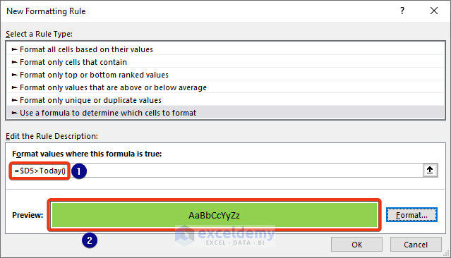
- Press the OK button.
Read More: Apply Conditional Formatting for Dates Older Than Today in Excel
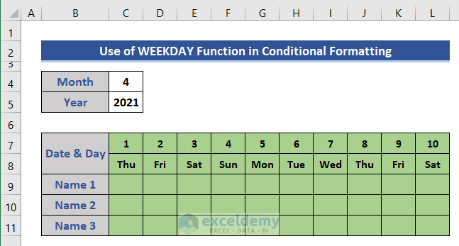
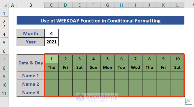
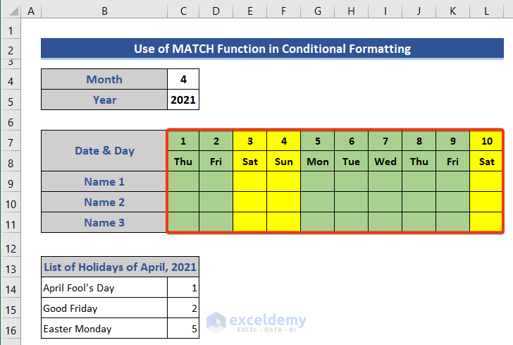
Example 3 – Using the WEEKDAY Function to Highlight Specific Days of a Week
We highlighted the weekends of the first two weeks of April 2021 in the calendar using the WEEKDAY function.
Steps:
- Select the cells you want to apply the conditional formatting on (In our case, C7:L11).
- Go to the New Formatting Rule window by following the steps of Example 2.
- Select the Use a formula to determine which cells to format rule type.
- Enter the following formula in the specified field.
=WEEKDAY(C$8,2)>5
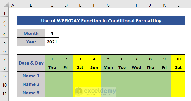
- Select the desired format by following the steps in Example 1.
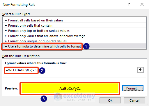
Explanation:
=WEEKDAY(C$8,2)>5 only returns a TRUE value when the days are Saturday (6) and Sunday (7) and formats the cells accordingly.
- Press the OK button.
Read More: Highlight Row with Conditional Formatting Based on Date in Excel
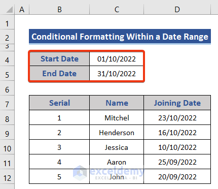
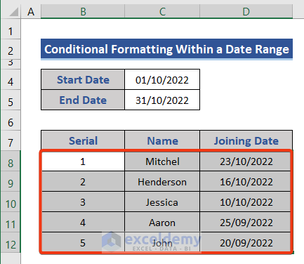
Example 4 – Highlight Dates Within a Date Range Using the AND Rule in Conditional Formatting
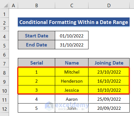
We have formatted the rows where the joining dates are between two different dates. We will highlight the cells with the joining date between the start and the end date.
Steps:
- Select the cells you want to apply the conditional formatting on (B8:D12).
- Go to the New Formatting Rule window by following the steps of Example 2.
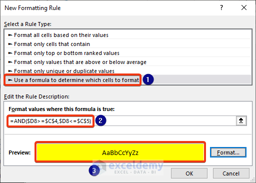
- Select the Use a formula to determine which cells to format rule type.
- Enter the condition/formula in the specified field
=AND($D8>=$C$4, $D8<=$C$5)
- Select the desired format by following the steps from Example 1.
Explanation:
=AND($D13>=$C$4, $D13<=$C$6) checks whether the dates in Column D are greater than the C4 cell’s date and less than the C6 cell’s date. If the date satisfies the conditions, then it formats the cell).
- Press the OK button.
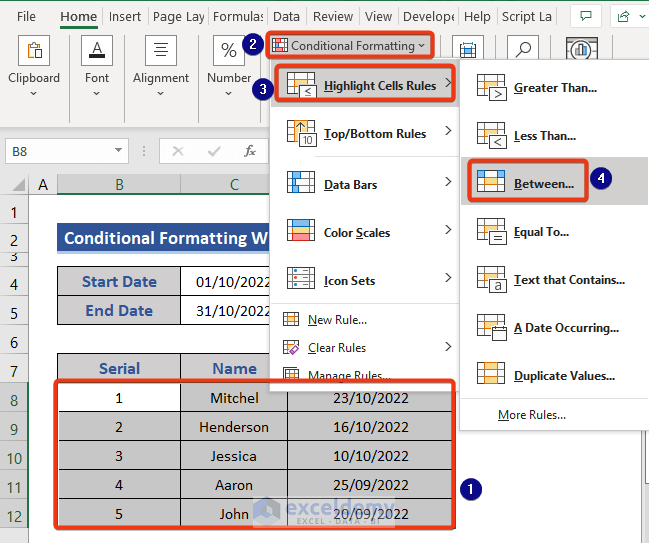
Alternate Method:
- Select the range B8:D12.
- Choose Highlight Cells Rules from the Conditional Formatting drop-down.
- Click on the Between option from the list.
- A dialog box will appear named Between.
- Put the cell reference of the start date on the box marked as 1 and the end date on the box marked as 2.
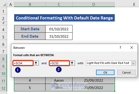
- Press the OK button.
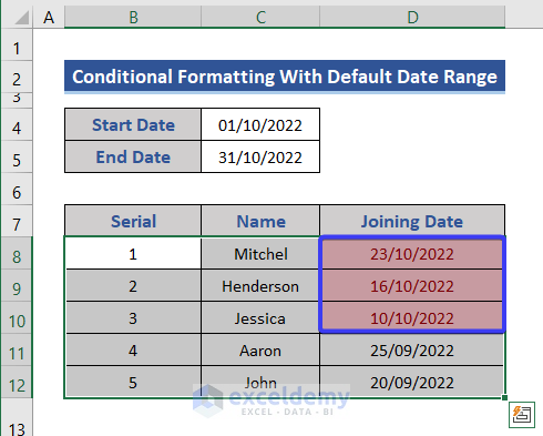
The first method modifies the color of the whole row based on the condition, but the alternative method is applicable to the cells only.
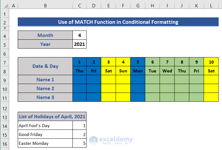
Example 5 – Highlight Holidays with the MATCH or COUNTIF Function in Conditional Formatting
Steps:
- Add a list of holidays of April 2021 to the dataset.
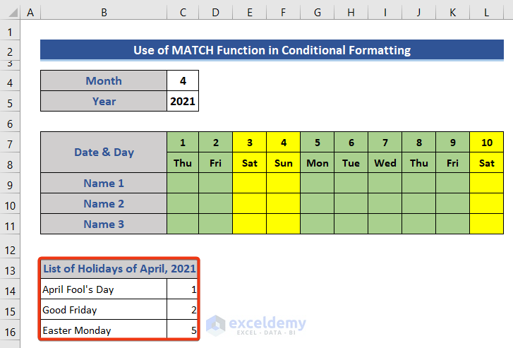
- Select the range C7:L11.
- Follow the steps of Example 2 and enter the following formula on the marked field.
=MATCH(C$7,$C$14:$C$16,0)
- Choose the desired color from the Format section.
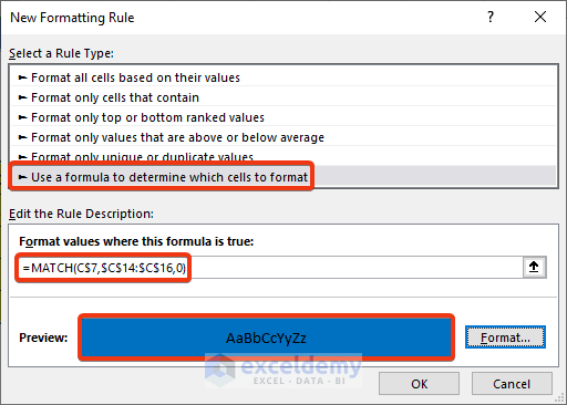
- Press the OK button.
- Here’s an alternative formula you can use:
=COUNTIF($C$14:$C$16,C$7)>0
Read More: How to Change Cell Color Based on Date Using Excel Formula
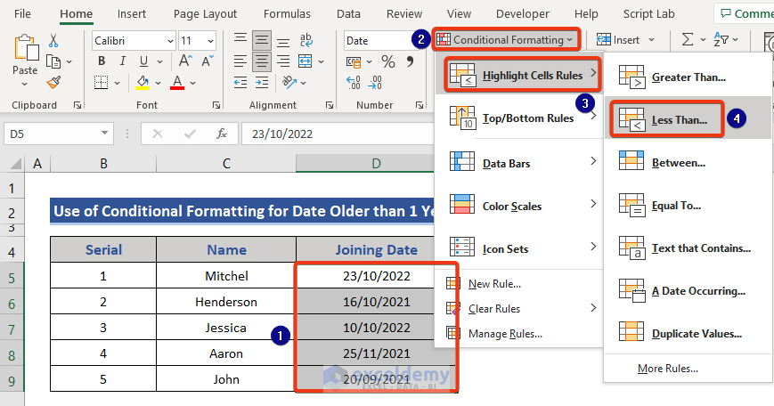
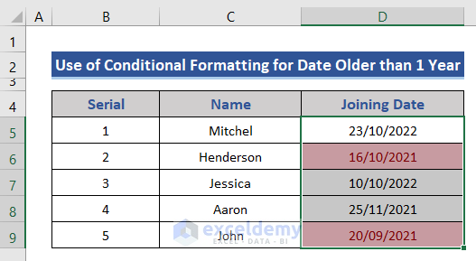
Example 6 – Excel Conditional Formatting Based on Date Older Than 1 Year
Steps:
- Select range D5:D9, which contains dates only.
- Select the Less Than option from the Highlight Cells Rules section.
- The Less Than window appears.
- Put the following formula:
=TODAY()-365
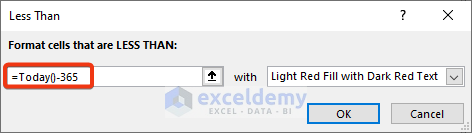
- Press the OK button.
Read More: Excel Conditional Formatting for Dates within 30 Days
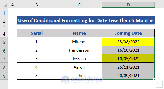
Example 7 – Excel Conditional Formatting Based on a Date Less Than 6 Months from Today
Steps:
- Select the range D5:D9.
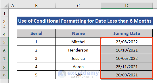
- Follow the steps of Example 2.
- Insert the following formula:
=DATEDIF($D5,TODAY(),''m'')<6
- Define the format of highlighted cells as shown in Example 1.
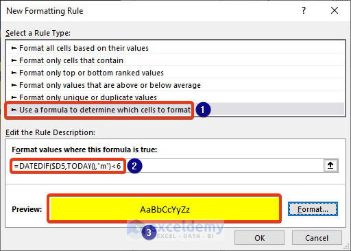
- Press the OK button.
Read More: Apply Conditional Formatting to Overdue Dates in Excel
Example 8 – Excel Conditional Formatting If It’s 15 Days After a Due Date
Steps:
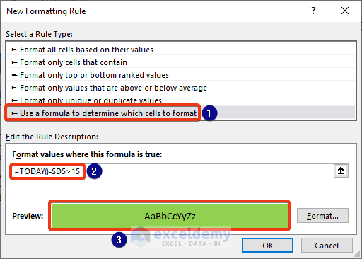
- Select the cells of the Joining Date column.
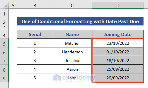
- Follow the steps of Example 2 and go to the New Formatting Rule section.
- Put the following formula in the box:
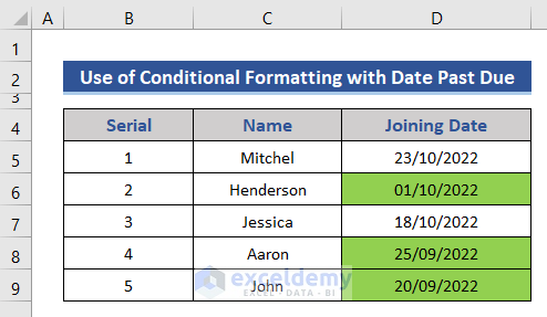
=TODAY()-$D5>15
- Choose the highlighting color from the Format option.
- Press the OK button.
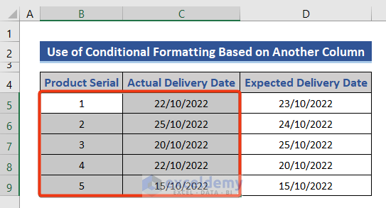
Example 9 – Conditional Formatting Based on the Date in Another Column
We will apply conditional formatting on the Actual Delivery Date column based on the Expected Delivery Date.
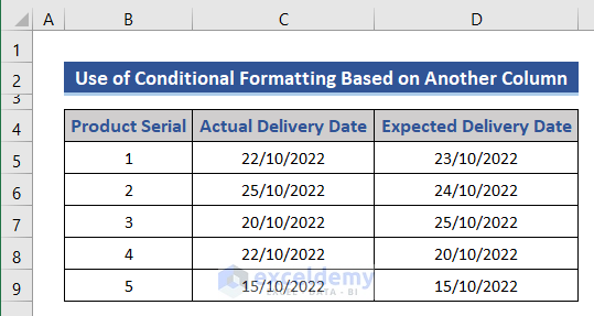
Steps:
- Select the range B5:C9.
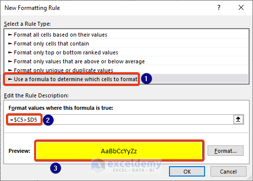
- Go to the New Formatting Rule section as shown in Example 2.
- Put the following formula in the box:
=$C5>$D5
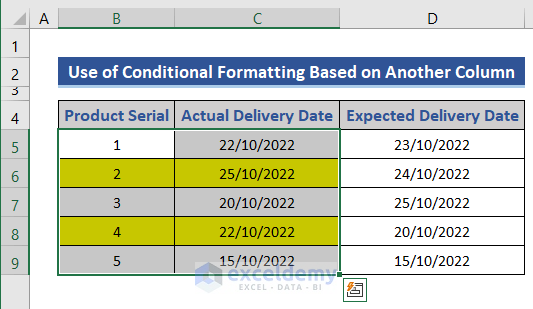
- Choose the desired cell color from the Format feature.
- Press the OK button.
Read More: Conditional Formatting Entire Column Based on Another Column in Excel
Download the Practice Workbook
Excel Conditional Formatting Based on Date: Knowledge Hub
- Highlighting Row with Conditional Formatting Based on Date
- Conditional Formatting Based on Date in Another Cell
- Apply Conditional Formatting for Dates Older Than Today
- Change Cell Color Based on Date Using Excel Formula
- Apply Conditional Formatting to Overdue Dates
- Excel Conditional Formatting for Dates Within 30 Days
<< Go Back to Conditional Formatting | Learn Excel
Get FREE Advanced Excel Exercises with Solutions!

This was super helpful, thank you
Hello SM,
You are most welcome. Thanks for your feedback and appreciation. Keep learning Excel with ExcelDemy!
Regards
ExcelDemy
Very informative, but I’m wondering if a rule can be developed to highlight a date cell one colour if the date is between 0 and 60 days less than TODAY(), and a different colour if the date is between 61 and 90 days less than TODAY().
Thanks.
Hello Ray,
Thank you for your kind words! Yes, you can create rules for this using conditional formatting and custom formulas. Here’s how you can set it up:
Highlight dates between 0 and 60 days less than TODAY():
1. Select your date range.
2. Go to Conditional Formatting > New Rule > Use a formula to determine which cells to format.
3. Enter this formula:
=AND(A1<=TODAY(), A1>=TODAY()-60)
4. Set your desired formatting and click OK.
Highlight dates between 61 and 90 days less than TODAY():=TODAY()-90)
Repeat the steps above with this formula:
=AND(A1
Apply a different formatting style for this rule.
Replace A1 with the first cell in your date range. These rules will work simultaneously to format cells based on your specified ranges. Let me know if you need further clarification!
Regards
ExcelDemy
Is it possible to do conditional formatting on weekend days, while using the “Long Date” Format (Sunday, April 6, 2025)?
Hello Rob,
Yes, it’s definitely possible to apply conditional formatting to weekend days even when using the “Long Date” format like “Sunday, April 6, 2025”. The formatting is based on the actual date value, not the display format. You can use a formula like:
=OR(WEEKDAY(A1)=1, WEEKDAY(A1)=7)
This checks if the date in cell A1 is a Saturday (7) or Sunday (1). Just apply this formula in the conditional formatting rule, and it will highlight weekends regardless of whether the date is shown in long or short format.
Regards
ExcelDemy