You can employ the Excel database functions to help you when using an Excel dataset. Sometimes, you may need to find the variance due to some specific criteria. Then, we will need the DVAR function. This article will show you how to use the DVAR function in Excel.
What Is Variance?
Variance is an assessment of a data set’s variability that shows how widely apart the different values are from one another. It is mathematically formulated as the average of the squared deviations from the average. Let’s have three numbers X1, X2, and X3, and the average of these three numbers is X̅. Therefore, the general formula of variance is given below.

- Firstly, we will calculate the average of all the numbers by applying the following formula.

- Therefore, we will find the differences between all the numbers from averages particularly by using this formula.

- After that, we will apply the variance formula to find the variance.

- Finally, you will see the output.

Introduction to DVAR Function
Objective
The objective of the Excel DVAR function is to obtain sample variance for matching records.
Syntax
Arguments Explanation
| Argument | Required/Optional | Explanation |
|---|---|---|
| Database | Required | The range of cells that you want to apply the criteria against. |
| Field | Required | The column to be used in the calculation. You can either specify the numerical position of the column in the list or the column label in double quotation marks. |
| Criteria | Required | The range of cells that contains your criteria. |
Version
- The DVAR function is available from Microsoft Excel 2000.
- Here, we will use Microsoft Excel 365.
DVAR Function in Excel: 2 Suitable Examples
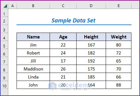
For only selected records, the Excel DVAR function determines the sample variance of a field in a database. It is one of the Database Functions. Here, we will demonstrate two examples of the DVAR function using Named ranges and Index in Excel. So, let’s have a sample data set.
Example 1: Using DVAR Function for Named Ranges in Excel
Here, we will use the DVAR Function for named ranges (Weight) for the following data set with specified criteria. So, to know this, you can follow the below steps accordingly.
Steps:
- Firstly, we have specified limits for age and height in columns G and C.
- Secondly, choose cell I5.
- Thirdly, write down the following formula with specific criteria.
- After that, press Enter.
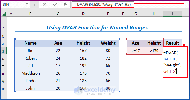
- Finally, you will get the following result of variance of weight.

Example 2: Applying DVAR Function by Index in Excel
Here, we will apply the DVAR Function by the index (4) for the following data set with specified criteria. So, to know this, you can follow the below steps accordingly.
Steps:
- Firstly, we have specified limits for age and height in columns G and C.
- Then, choose cell I5.
- After that, write down the following formula with specific criteria.
- So, press Enter.
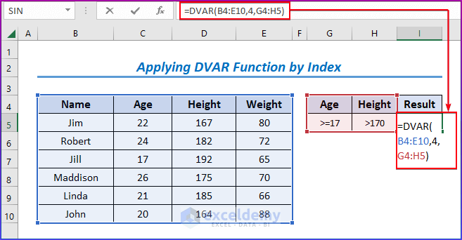
- Therefore, you will get the following output of variance of weight.

Download Practice Workbook
You may download the following Excel workbook for better understanding and practice it by yourself.
Conclusion
In this article, we’ve covered two suitable examples of how to use the DVAR function in Excel. We sincerely hope you enjoyed and learned a lot from this article. If you have any questions, comments, or recommendations, kindly leave them in the comment section below.
<< Go Back to Excel Functions | Learn Excel
Get FREE Advanced Excel Exercises with Solutions!
