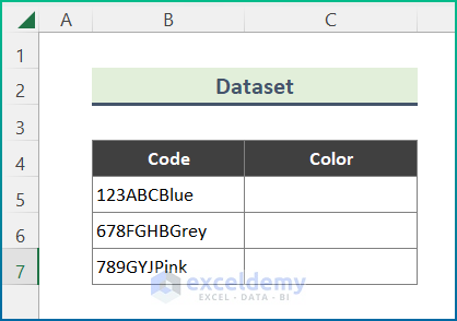
Some spreadsheets like the following sample dataset require us to trim data from the left. Here, we need to trim the Color from the given Product Code.
Method 1 – Using the RIGHT Function to Trim Characters in Excel
Steps:
- Enter the following formula to separate the color from the code.
=RIGHT(B5,4)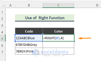
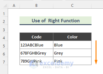
- After entering the formula, the color Blue will be separated.
- Use the Fill Handle (+) to copy the formula to the rest of the cells.
Read More: How to Trim Right Characters and Spaces in Excel
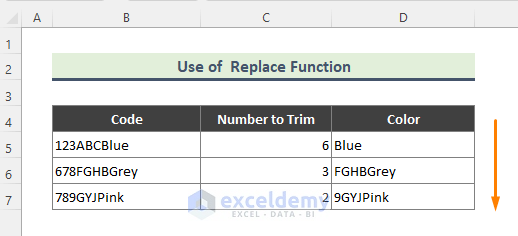
Method 2 – Using the REPLACE Function to Remove Selected Characters from the Left Column
Steps:
- Enter the following Formula:
=REPLACE(B5,1,C5,"")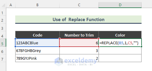
- You should now see the following:
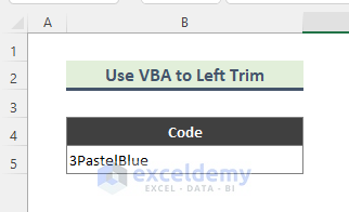
Method 3 – Using VBA to Trim Selected Characters from the Left Column
This method works if you do not want to use a formula or function.
Steps:
- Following is the string we want to trim:
- Right-click on the sheet name and select the View Code option to view the VBA window.
- Type the following code in the Module.
Option Explicit
Sub GetString()
Dim str1 As String
str1 = "3PastelBlue"
MsgBox Right(str1, 10)
End Sub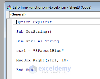
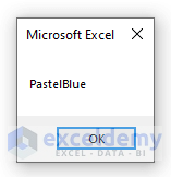
- Run the code
Method 4 – Using RIGHT and LEN Functions to Remove Selected Characters from the Left Column
The LEN function returns the number of characters in a text string.
Steps:
- Enter the following formula.
=RIGHT(B5,LEN(B5)-C5)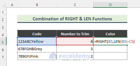
Breakdown of the Formula:
- LEN(B5)
Here, the LEN function returns the number of characters in a text string.
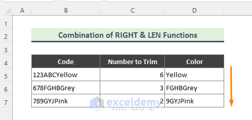
- RIGHT(B5,LEN(B5)-C5)
In this formula, the number of characters trimmed from the left is subtracted from the whole string. The formula will return the string trimmed from the left.
- This is what you will see:
Method 5 – Using a Combination of FIND, MID, TRIM & LEN Functions to Remove Selected Characters from the Left Column
Steps:
- Enter the following formula:
=MID(B5,FIND(MID(TRIM(B5),1,1),B5),LEN(B5))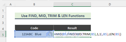
Breakdown of the Formula:
- LEN(B5)
This formula will return the number of characters in Cell B5.
- TRIM (B5)
The TRIM function removes all spaces from B5 except for single spaces between words.
- MID(TRIM(B5),1,1)
The MID function returns characters from the middle of B5, given the starting position and length.
- FIND(MID(TRIM(B5),1,1)
The FIND function returns the starting position of one text string within another text string. Here the formula returns the position of the character we found in the previous procedure.
- MID(B5,FIND(MID(TRIM(B5),1,1),B5),LEN(B5))
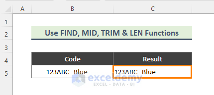
Applying the formula with another MID function will erase the spaces from only the left side of the string.
- You will see the output as shown below:
Read More: How to Trim Spaces in Excel
Method 6 – Using a Combination of REPLACE, LEFT, FIND & TRIM to Remove Selected Characters from the Left Column
Steps:
- Type the following formula:
=REPLACE(B5,1,FIND(LEFT(TRIM(B5),2),B5)-1,"")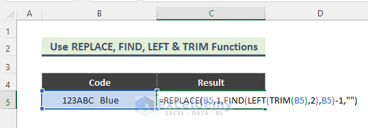
Breakdown of the Formula:
The combination of the FIND, LEFT and TRIM functions helps us to calculate the position of the first space character in the string; spaces towards the left side of the string. Here, we passed the formula through REPLACE function. As a result, the leading spaces of the string were replaced with no blank (“”). The formula will erase only the leading spaces from the string.
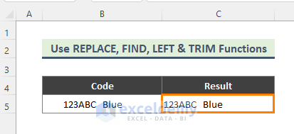
- The result is:
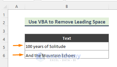
Method 7 – Using VBA to Trim Characters from the Left Column
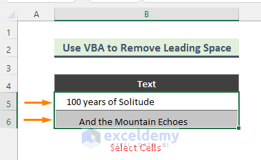
Leading spaces can also be deleted using the VBA.
Steps:
- Select the cells with leading spaces.
- Right-click on the sheet name, and select the View Code option to bring up the VBA window.
- In the Module, write the following code:
Option Explicit
Sub TrimExample1()
Dim Cell As Object
Dim Rg As Range
Set Rg = Selection
For Each Cell In Rg
Cell.Value = Trim(Cell)
Next Cell
End Sub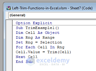
- Run the code.
Download Practice Workbook
You can download the practice workbook that we’ve used to prepare this article.
Related Articles
<< Go Back to Excel TRIM Function | Excel Functions | Learn Excel
Get FREE Advanced Excel Exercises with Solutions!
