Sometimes data cells may have additional characters attached to the right which is not required.
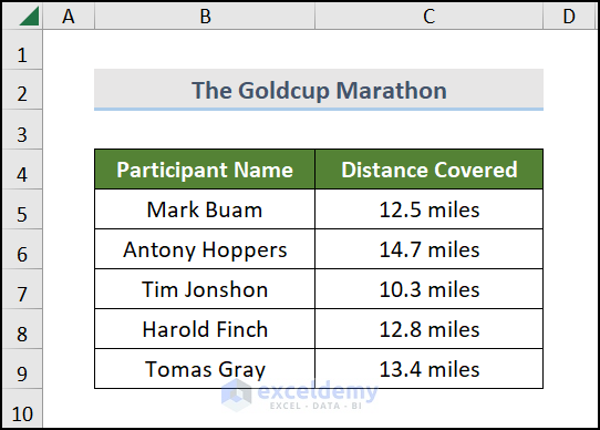
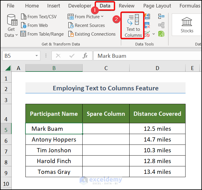
In the sample dataset the Distance covered by different participants at a marathon is recorded.
There are some spaces at the end of each Participant Name and the cells in the Distance Covered column have the numerical values as well as the unit – miles. We will trim the spaces and the unit from the right.
Method 1 – Utilizing TRIM Function to Remove Extra Spaces
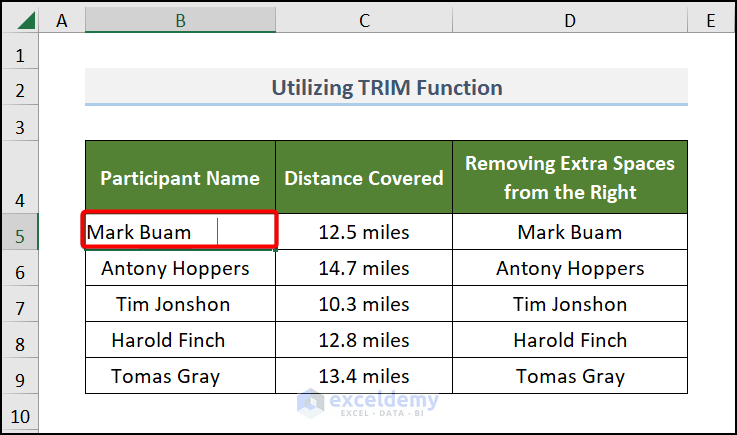
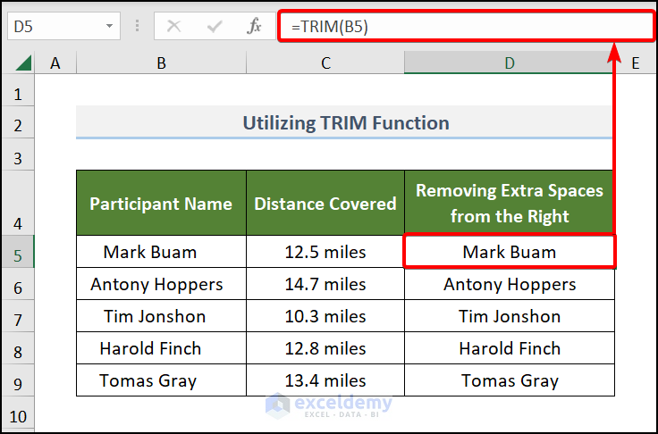
Type the following formula in an empty cell (D5)
=TRIM(B5)Press ENTER to remove all the extra spaces and use the Fill Handle to drag it down to the other cells.
Read More: How to Trim Spaces in Excel
Method 2 – Employing Text to Columns Feature to Trim Right Spaces
This method will require a spare column at the right of the column from where you will remove the spaces.
Steps
- Insert a column right to the column from where you will remove the space.

- Go to Data tab >> select Text to Columns under the Data Tools group.
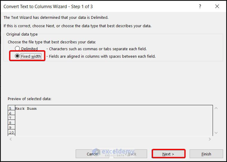
- A Text to Column Wizard window will appear. Select Fixed Width and click on Next.
- In the second screen, move the vertical line to the end of the data and select Next.
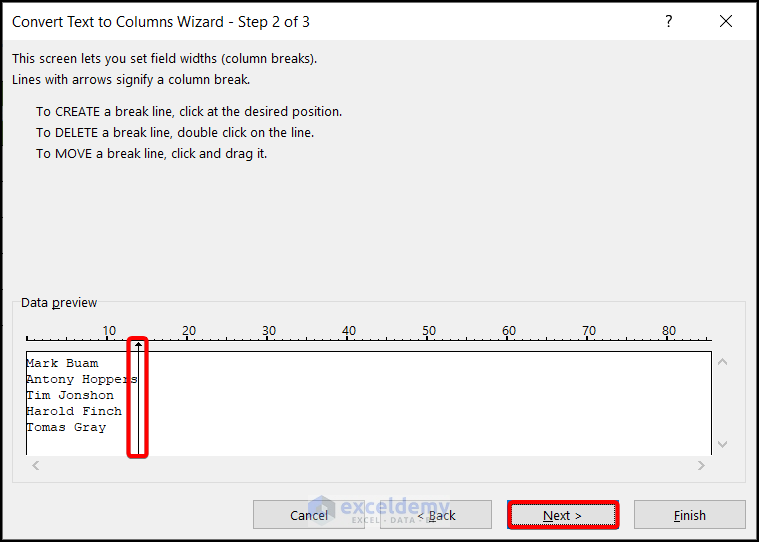
- All of the data is highlighted in black.
- Select Finish.
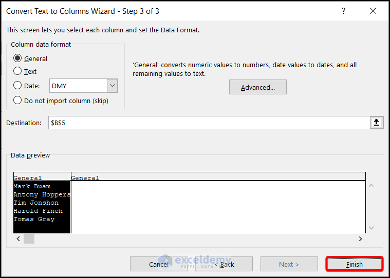
- A confirmation window will appear. Press OK.
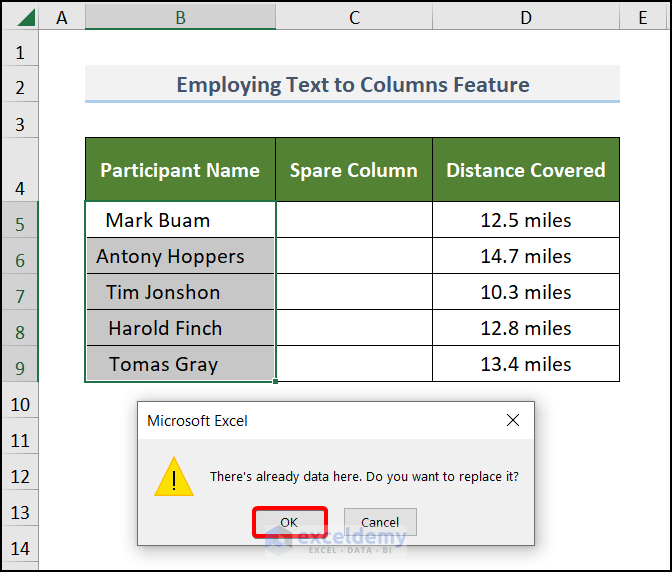
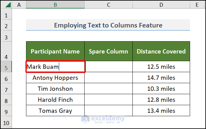
There are now no spaces to the right end of your dataset.
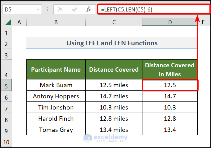
Method 3 – Using LEFT and LEN Functions to Trim Right Characters
- Type the following formula in an empty cell (D5).
=LEFT(C5,LEN(C5)-6)The LEFT function indicates that the formula will return the characters of the selected cell, C5 from the LEFT, and LEN(C5)-6 portion indicates that the last 6 characters from the total length of cell C5 are not to be returned.
- Press ENTER.
- Use the Fill handle to drag the formula to the other cells.

Read More: How to Trim Part of Text in Excel
Method 4 – Applying VALUE, LEFT, and LEN Functions
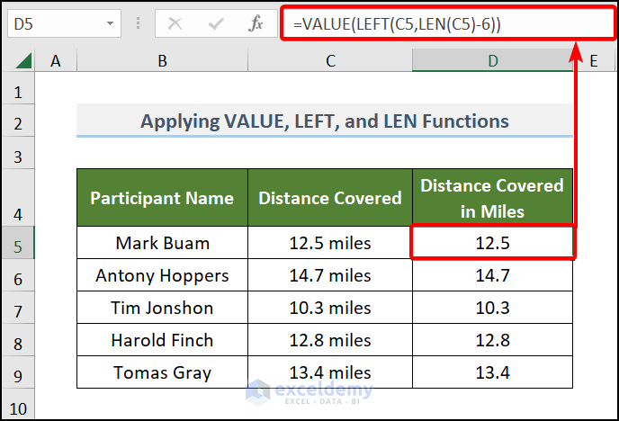
To get the numeric value after trimming the right characters, type the following formula in cell D5,
=VALUE(LEFT(C5,LEN(C5)-6))The VALUE function will convert the return of the LEFT function into numeric values.
- Press ENTER. The formula has trimmed the right characters.
- Use the Fill handle to drag the formula to the other cells.
Method 5 – Trim Right Characters Incorporating VBA Macros
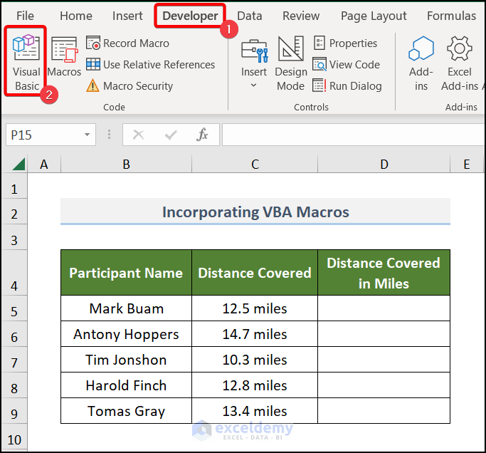
- Navigate to the Developer tab >> choose Visual Basic. Alternatively, you can press the ALT+F11 keys to open the Visual Basic editor window.
- Go to the Insert tab >> Module >> Module 1.
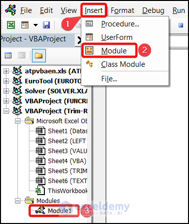
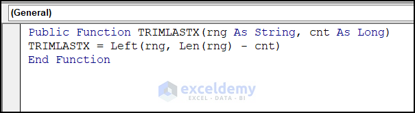
- Insert the following code in the Module 1 window.
Public Function TRIMLASTX(rng As String, cnt As Long)
TRIMLASTX = Left(rng, Len(rng) - cnt)
End Function
The code will create a custom function named TRIMLASTX which will trim a defined number of characters from the right side of the selected cell.
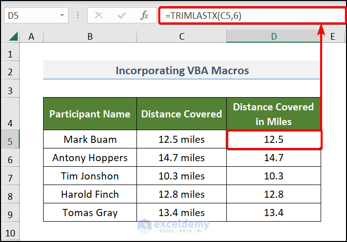
- Close the VBA window and type the following formula in cell D5.
=TRIMLASTX(C5,6)- C5 is the selected cell and 6 indicates the number of characters that will be removed.
- Press ENTER.
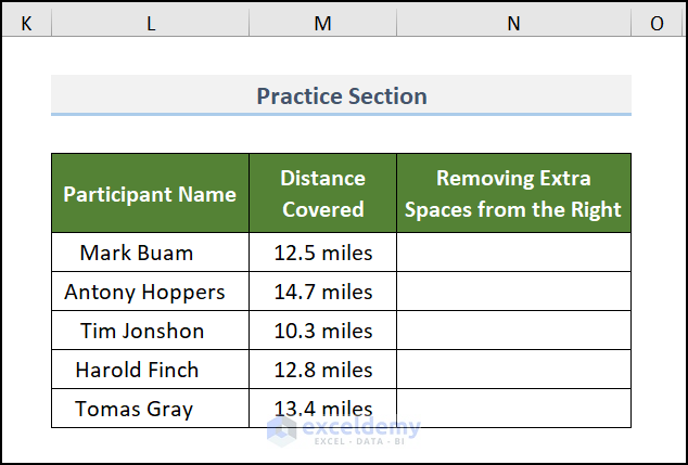
Practice Section
Download Practice Workbook
Further Readings
<< Go Back to Excel TRIM Function | Excel Functions | Learn Excel
Get FREE Advanced Excel Exercises with Solutions!

both trim and text to columns did not work i have a data set like yours in column A Which has an uneven amount of characters, but the same number of space to the right (2 spaces) so text to columns wouldn’t work for all of them and trim didn’t seem to work properly any other ideas to just have excel remove 2 characters from the right?
Hi TONY!
We checked the Excel file. It is working fine for an even and uneven amount of characters. Make sure the TRIM function and the text to the column are entered correctly. We suggest you download the file and practice there. If you are unable to solve your problem, you can also share your Excel file with us.
Thank you for being with us.
Regards
Md. Abdur Rahim Rasel(Exceldemy Team)