The MATCH function in Excel is a very useful function to find out exact or approximate data matches in Excel. However, you may have trouble choosing the match type in the function argument. But no worries! Just follow the article below. All your problems regarding the Excel MATCH function match type will be solved. Stay connected.
Introduction to MATCH Function in Excel
The MATCH function in Excel is used to find the relative position of a specified value within a range of cells. It returns the position of the first occurrence of the value in the range, counting from the top or leftmost cell.
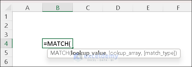
- Syntax:
=MATCH(lookup_value,lookup_array,[match_type])
- Arguments Explanation:
| Argument | Required/Optional | Explanation |
|---|---|---|
| lookup_value | Required | The value to match in the array |
| lookup_array | Required | A range of cells or an array reference where to find value |
| match_type | Optional | Specifies how Excel matches lookup_value with values in lookup_array. Here, 1 = exact or next smallest, 0 = exact match and -1 = exact or next largest |
- Return Value:
Returns the lookup value’s relative position.
- Available Version:
Workable from Excel 2003.
Excel MATCH Function Match Type: 3 Examples with Greater/Less Than & Exact Match
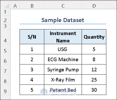
To illustrate, we will use a sample dataset. For instance, the following dataset shows the instruments available in a healthcare center and their corresponding quantity.
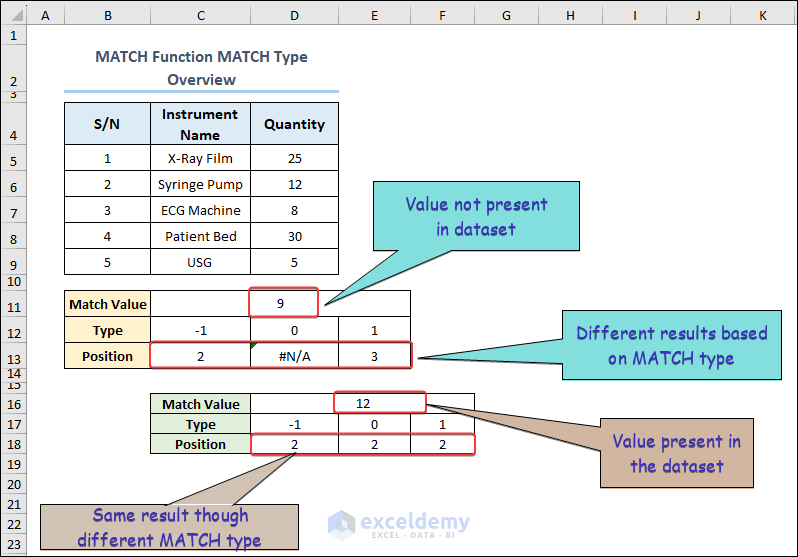
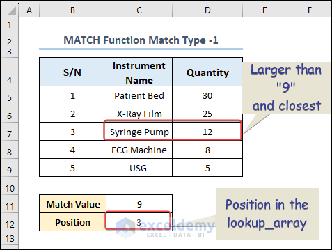
1. Match Type -1: Finding the Smallest Value Greater Than or Equal to Lookup Value
When you use match_type “-1”, first you should sort the lookup_array in descending order. Otherwise, you may get a result that is not predictable. Let us see how to use match type “-1” in the above dataset.
In the dataset, we want to check a value(9) that is not present in the dataset but the formula would return a value that is larger than the value and closest to the input value.
📌 Steps:
- Apply the following formula to cell C12.
=MATCH(C11,D5:D9,-1)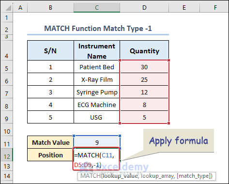
- Hit “ENTER” to get the result.
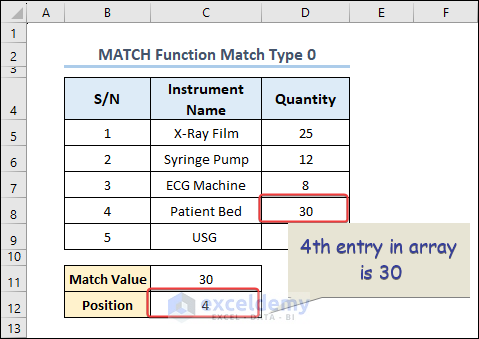
2. Match Type 0: Finding the Exact Match
In this stage, you may ask how we can use the MATCH function for an exact match. The answer is just to use “0” in the match type. You will be done. We will use the MATCH function in 2 cases. The first one is a simple case but in the second case, we will use the “Wildcard” character in the MATCH function.
2.1 Exact Match for Full String
Suppose you need to find out where the value “30” is located in the lookup_array. Just follow the simple steps below.
📌 Steps:
- Apply the following formula in cell C12.
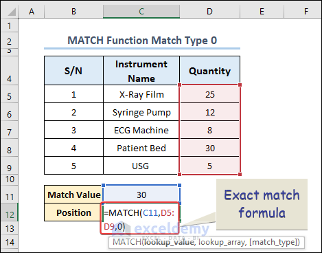
- Now you will get the result just by hitting ENTER.
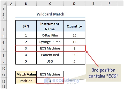
2.2 Matching Partial Texts with Wildcards
It is possible to match a partial text and find out the position in your dataset. Suppose, you want to find out the position of the “ECG Machine” in the lookup_array.In the formula of the MATCH function, use the wildcard ” EC*” instead of the full form to find the position of the text.
📌 Steps:
- Write the following formula in cell C12.
=MATCH("EC*",C5:C9,0)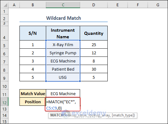
- If you wish to see the output, just hit ENTER. You will see an output like the image below.
Read More: [Fixed!] Excel MATCH Function Not Working
3. Match Type 1 (Default Type): Finding the Largest Value Less Than or Equal to Lookup Value
The default match type of the MATCH function is 1. When you don’t mention the match type in the formula, it will automatically set the value to 1.
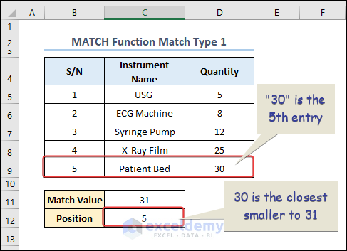
Let us find the closest large and at the same time smaller than the value “31” in the array.
📌 Steps:
- We are going to write down the following formula in C12.
=MATCH(C11,D5:D9,1)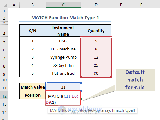
- Now, hit ENTER and get the desired output.
How to Perform Case-Sensitive Match in Excel Combining with EXACT Function
The MATCH function returns matches found irrespective of the case. However, it is possible to modify the code to make it case-sensitive. We will combine the MATCH function with the EXACT function in the following example and perform case sensitive match. Follow the steps described below.
📌 Steps:
- In order to combine 2 formulas, write down the following code in cell C12.
=MATCH(TRUE,EXACT(C5:C9,C11),0)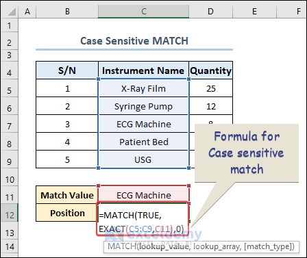
- Then hit ENTER and get the output at the desired cell.
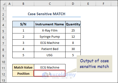
To check whether the formula works properly, replace any of the lowercase words with the corresponding uppercase. The output will be #N/A.
🔎 Formula Explanation:
EXACT(C5:C9,C11)
- Returns an array which is: {FALSE,FALSE,TRUE,FALSE,FALSE}.
MATCH(TRUE,EXACT(C5:C9,C11),0)
- Check which entry in the array is TRUE.
- The exact match since match_type is “0”.
- Finds that 3rd entry in the array is TRUE. So, returns 3 in output.
Frequently Asked Questions
- What does the MATCH function do in Excel?
The MATCH function in Excel searches for a specified value in a specified array and returns the position of that value within the array.
- What is the purpose of the match_type argument in the MATCH function?
The match_type argument in the MATCH function specifies the type of match that you want to perform. There are three possible values for match_type: 1, 0, and -1.
- Can the MATCH function return multiple matches?
No, the MATCH function returns only the position of the first matching value that it finds in the lookup_array.
Things to Remember
- The MATCH function is not case-sensitive.
- The function returns a #N/A error in case of no match.
- The MATCH function works only with text having 255 characters in length.
- When there is more than one match, the function returns the first match it finds.
- If the match_type is “-1” or “1”, the lookup_array should be sorted first.
Download Practice Workbook
You may download the following workbook to practice yourself.
Conclusion
You are at the end of the article Excel MATCH function match type. To summarize, we have discussed examples of different match types in the MATCH function. Hopefully, these examples were helpful for you. Moreover, do let us know if you have any further queries.
<< Go Back to Excel MATCH Function | Excel Functions | Learn Excel
Get FREE Advanced Excel Exercises with Solutions!
