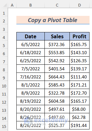
In the dataset, you will see a shop’s Sales and Profit information on random days from June to August. We will use this data to create a Pivot Table and show you how to copy it.
Before copying, we need to create a Pivot Table using the data.
Steps:
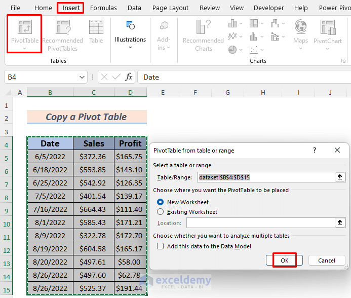
- Select the range of the data (B4:D15) and go to Insert >> Pivot Table.
- The Pivot Table window will show up.
- Select the option where you want your Pivot Table to be created and click OK. In this case, I selected a New Worksheet so that the Pivot Table will appear in a new worksheet.
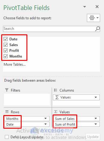
- Drag the PivotTable Fields to the PivotTable Area.
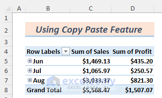
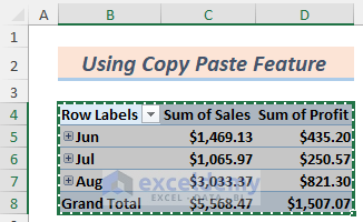
Method 1 – Using the Copy-Paste Feature to Copy a Pivot Table
Copy the table.
Steps:
- Select the PivotTable data and press CTRL+C to copy it.
- Paste the Pivot Table into another sheet. This step is very important because if you paste the Pivot Table into the same sheet, the original Pivot Table won’t work, as Excel does not allow one Pivot Table to overlap another. Both Pivot Tables work perfectly if you paste them into a different sheet.
You can see that there are various Paste Options, and you should choose any of them according to your purpose.
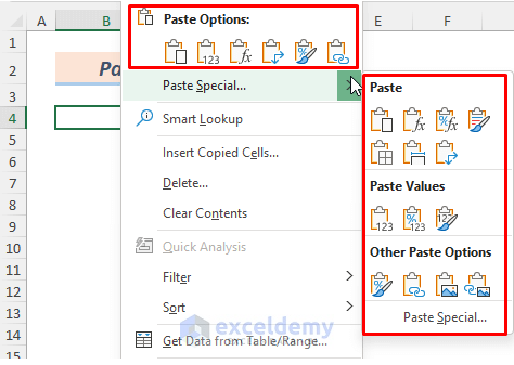
- Paste it (press CTRL+V).
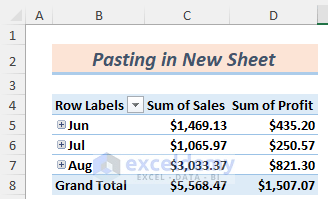
- Both these Pivot Tables work correctly.
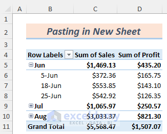
- Click on the Plus (+) icon beside the month of June in the original Pivot Table. You will see the detailed Sales and Profit.
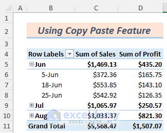
- Do the same operation on the copied Pivot Table. You will see the same data on the Pivot Table.
Method 2 – Applying a Clipboard to Copy a Pivot Table
Steps:
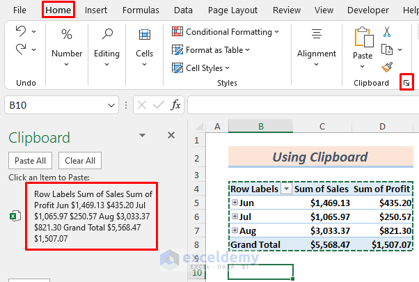
- Select the Pivot Table and press CTRL+C.
- Click on the marked icon on the clipboard. You will find this ribbon in the Home tab.
- Select a cell where you want to paste the Pivot Table.
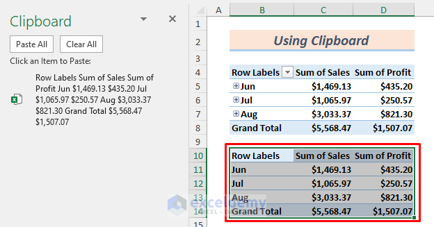
- Click on the marked item in the Clipboard.
- You will see the Pivot Table data pasted in the Excel worksheet.
Download the Practice Workbook
How to Copy a Pivot Table in Excel: Knowledge Hub
- How to Copy and Paste Pivot Table Values with Formatting in Excel
- Copy Pivot Table Data to Another Worksheet Without Pivot in Excel
<<Go Back to Pivot Table in Excel | Learn Excel
Get FREE Advanced Excel Exercises with Solutions!
