How to Copy and Paste Pivot Table Values with Formatting in Excel

If you copy a pivot table and then paste it in the usual manner (CTRL +C / CTRL + V), you will get the pivot table but not necessarily with the formatting of the values preserved. This article will describe 3 ways to copy and paste pivot table values including the formatting.

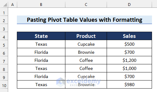
We’ll create a pivot table from the following dataset of sales information, then copy and paste the values with formatting intact.

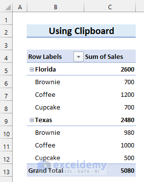
Method 1 – Using the Clipboard

First we’ll insert the pivot table to be copied. Then, we’ll format it. Then we’ll use the Clipboard to copy and paste it.

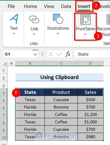
Step 1 – Insert Pivot Table

• Select the data from which to make the pivot table.
• Go to the Insert tab on the Ribbon.
• Select PivotTable.

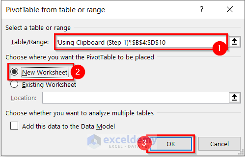
The PivotTable from table or range will appear, and the Table/Range will be selected automatically.

• Select New Worksheet.
• Click OK.

A PivotTable will be inserted into a new Excel sheet. Now, we add fields to this PivotTable.

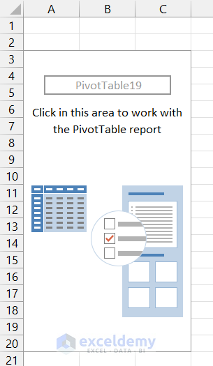
• Click any cell of the table.

The PivotTable Fields Task Pane will appear on the Right side of the screen.

• Select and drag the fields you want as Rows.
• Select and drag the field you want as Values.

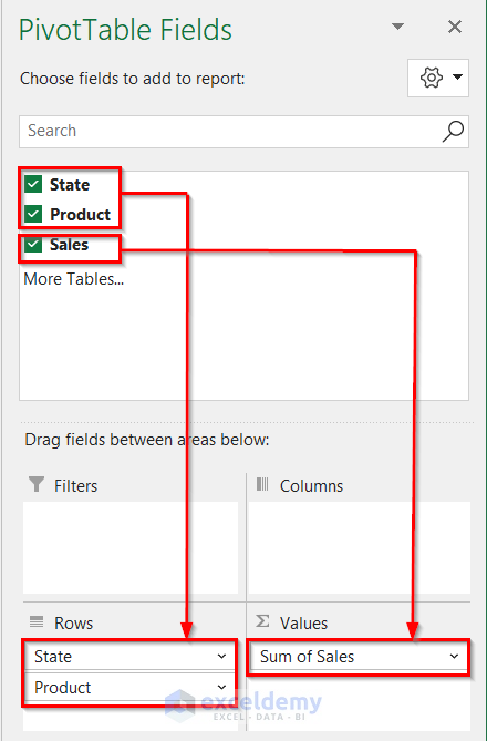
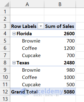
The PivotTable looks like this:

Step 2 – Format Pivot Table in Excel

• Format the sheet like in the following image to give it a better look.

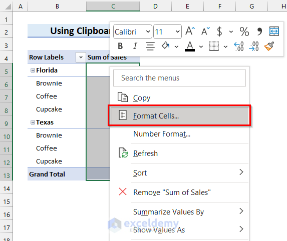
To change the format of the cells:

• Select the cells and right-click.
• Select Format Cells from the context menu.

The Format Cells dialog box will appear.

• Select the Category you want, for example Currency.
• Click OK.

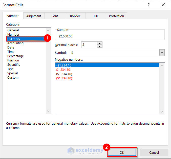
The format is changed to Currency.

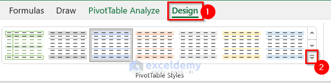
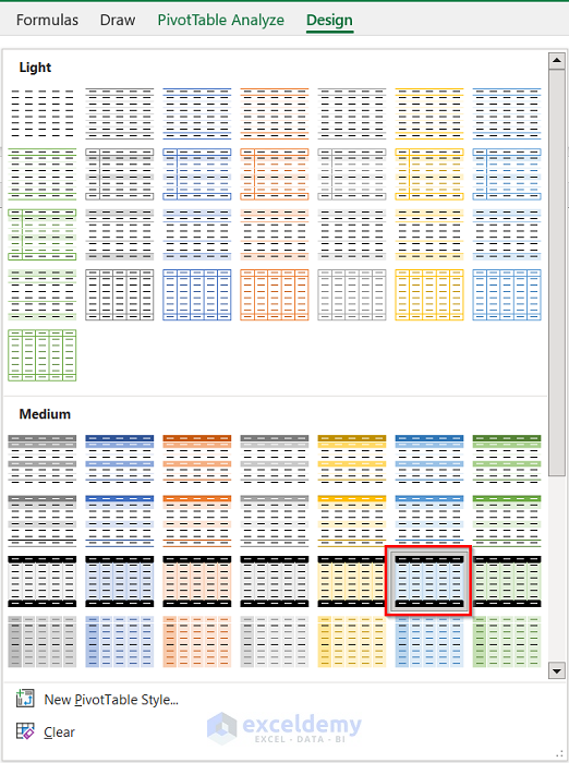
Next, we change the Style of the PivotTable:

• Select the PivotTable.

• Go to the Design tab.
• Click on the button marked in the following image.

A drop-down menu will appear.

• Select the Style you want. Here, the marked Style for the PivotTable.

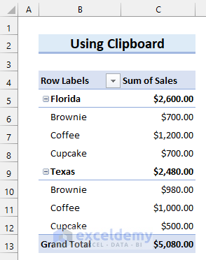
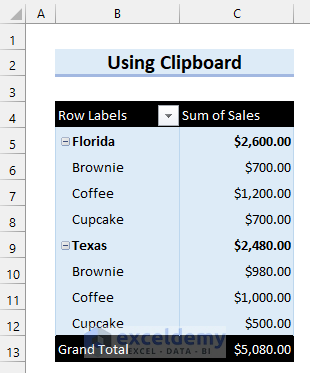
The formatted PivotTable now looks something like this:

Step 3 – Copy Pivot Table with Formatting

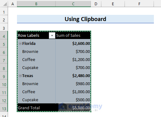
Now we’ll copy our formatted pivot table:

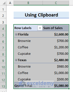
• Select the PivotTable.
• Press Ctrl + C to copy it.

• Go to the Home tab.
• Click on the icon marked below to open the Clipboard.

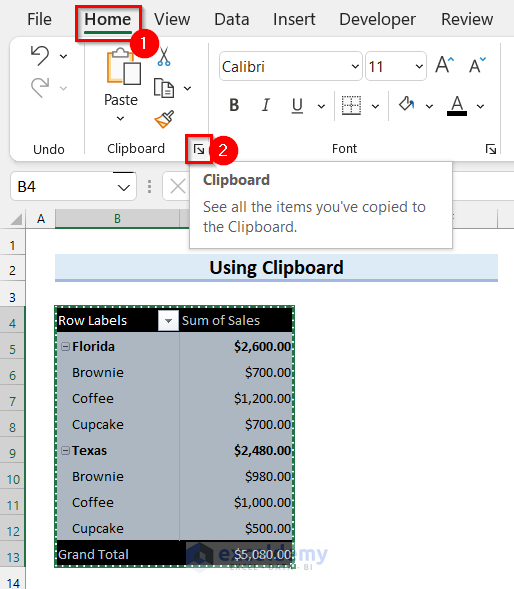
The Clipboard will appear on the left side of the screen.

• Select the cell to paste the PivotTable.
• Select the PivotTable from the Clipboard.

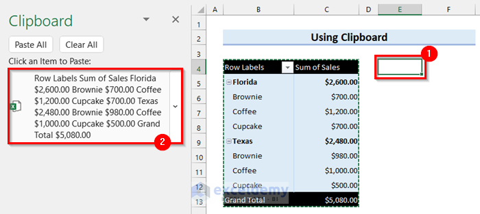
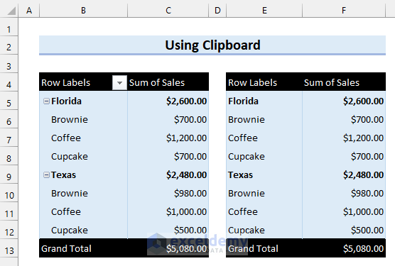
The PivotTable values are copied with their formatting.

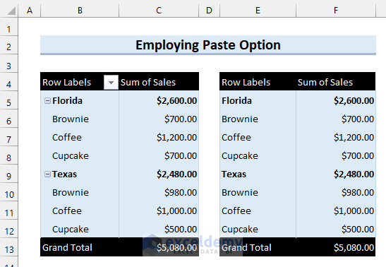
Method 2 – Using Paste Option

Steps:

• Select the PivotTable.
• Press Ctrl + C to copy it.
• Select the cell to paste the pivot table values. Here, cell E4.
• Go to the Home tab.
• Click on the drop-down option for Paste.
• Select Values & Source Formatting.

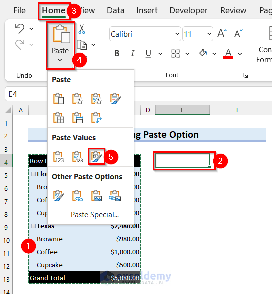
The values in the PivotTable are pasted as is.

• Click on the drop-down menu to paste again.
• Select Formatting.

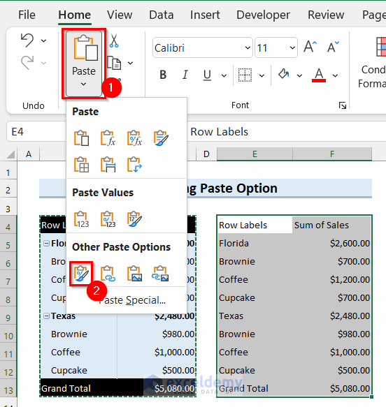
• The values are copied with their formatting intact.

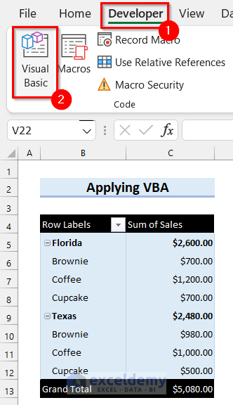
Method 3 – Using Excel VBA

Here, we will apply VBA code to paste the values into a new worksheet with formatting intact.

Steps:

• Go to the Developer tab.
• Select Visual Basic.

The Visual Basic Editor window will appear.

• Select the Insert tab.
• Select Module.

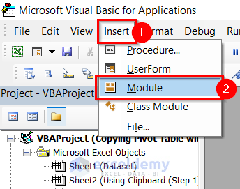
A module will appear.

• Enter the following code in the module:

Sub Paste_PT_with_Format()
Dim my_worksheet As Worksheet
Dim pivot_table As PivotTable
Dim pvt_tbl_rng As Range
Dim pvt_tbl_rngA As Range
Dim copy_rng As Range
Dim copy_rng2 As Range
Dim pt_top_row As Long
Dim pt_rows As Long
Dim pt_rows_page As Long
Dim message_spaces As String
On Error Resume Next
Set pivot_table = ActiveCell.PivotTable
Set pvt_tbl_rngA = pivot_table.PageRange
On Error GoTo errHandler
If pivot_table Is Nothing Then
    MsgBox "Excel Can't Copy PitotTable"
    GoTo exitHandler
End If
If pivot_table.PageFieldOrder = xlOverThenDown Then
  If pivot_table.PageFields.Count > 1 Then
    message_spaces = "Spaces with filters." _
      & vbCrLf _
      & "Can't copy filters."
  End If
End If
Set pvt_tbl_rng = pivot_table.TableRange1
pt_top_row = pvt_tbl_rng.Rows(1).Row
pt_rows = pvt_tbl_rng.Rows.Count
Set my_worksheet = Worksheets.Add
Set copy_rng = pvt_tbl_rng.Resize(pt_rows - 1)
Set copy_rng2 = pvt_tbl_rng.Rows(pt_rows)
copy_rng.Copy Destination:=my_worksheet.Cells(pt_top_row, 1)
copy_rng2.Copy _
  Destination:=my_worksheet.Cells(pt_top_row + pt_rows - 1, 1)
If Not pvt_tbl_rngA Is Nothing Then
    pt_rows_page = pvt_tbl_rngA.Rows(1).Row
    pvt_tbl_rngA.Copy Destination:=my_worksheet.Cells(pt_rows_page, 1)
End If
my_worksheet.Columns.AutoFit
If message_spaces <> "" Then
  MsgBox message_spaces
End If
exitHandler:
    Exit Sub
errHandler:
    MsgBox "Excel Can't Copy PitotTable"
    Resume exitHandler
End Sub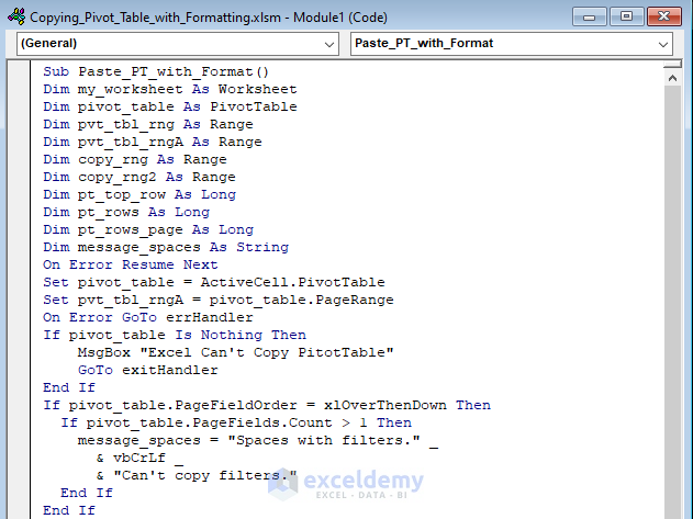

How Does the Code Work?

• Save the code and go back to your worksheet.
• Select the PivotTable.
• Go to the Developer tab.
• Select Macros.

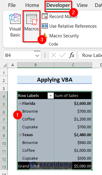
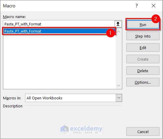
The Macro dialog box will appear.

• Select Paste_PT_with_Format as the Macro name.
• Click Run.

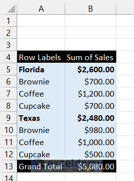
We have copied and pasted the values of the PivotTable with formatting in a new worksheet.

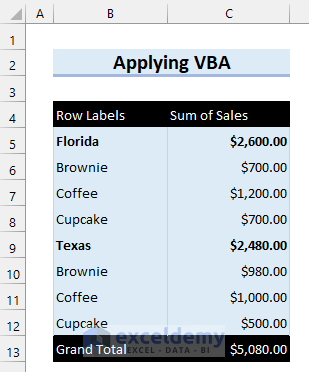
After some additional formatting, the output looks like this:

Things to Remember

• When working with VBA, save the Excel file as Excel Macro-Enabled Workbook. Otherwise, the VBA code will not work properly.

Download Practice Workbook

Related Articles

• Copy Pivot Table Data to Another Worksheet Without Pivot in Excel

<<Go Back to How to Copy Pivot Table| Pivot Table in Excel | Learn Excel