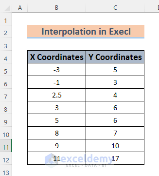
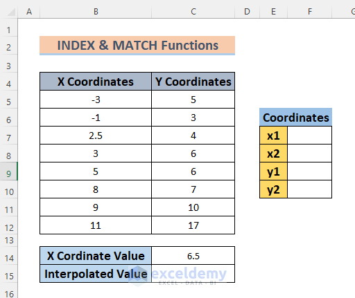
In the dataset, we have some X Coordinates and Y Coordinates. We’ll interpolate the value for given coordinates.
Method 1 – Using the FORECAST or FORECAST.LINEAR Function to Interpolate Between Two Values in Excel
Steps:
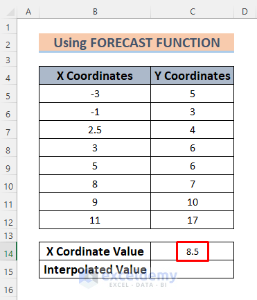
- Make new rows for the value you want to interpolate. We want to interpolate between 8 and 9, so we chose a value of 8.5 and put it in C14.
- Use the following formula in cell C15.
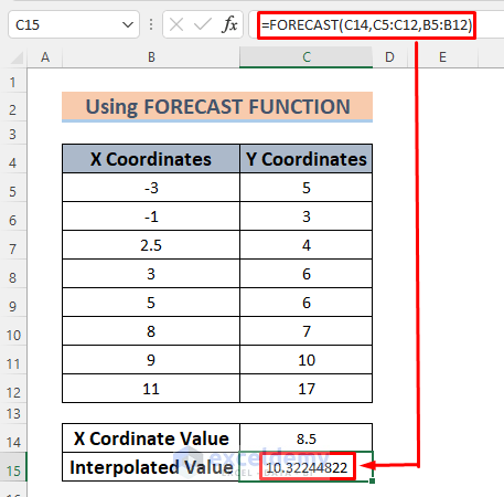
=FORECAST(C14,C5:C12,B5:B12)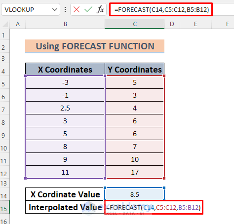
The FORECAST function determines the interpolated value in cell C15 via linear regression. It works on the ranges B5:B12 (as known_Xs) and C5:C12 (as known_Ys).
- Hit the Enter button.
- You can also use the following function:
=FORECAST.LINEAR(C14,C5:C12,B5:B12)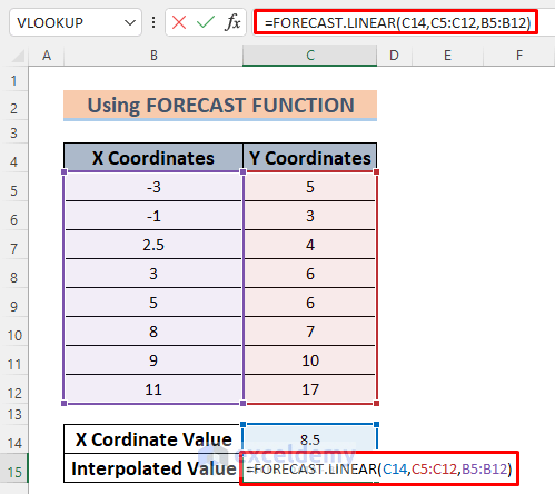
- Hit Enter.

The FORECAST function is getting deprecated by FORECAST.LINEAR, so it might not be available for newer Excel versions.
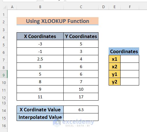
Method 2 – Combining Excel XLOOKUP and FORECAST Functions to Interpolate Between Two Values
Suppose we want to interpolate for the x-value 6 in B9:C10.
Steps:
- Modify the dataset to place the coordinates.
- Use the following formula in cell F7.
=XLOOKUP(C14, B5:B12,B5:B12,,-1,1)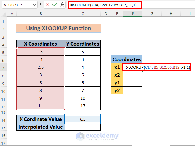
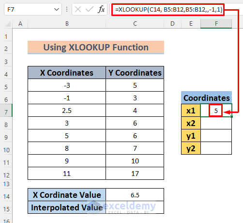
The XLOOKUP function looks up the value in C14, searches for this value in the range B5:B12, and returns the value which is adjacently smaller than 6.5 as it cannot find this exact value in that range and we put -1 in this regard. We get x1 as 5.
When we need a value adjacently larger than 6.5, we use ‘1’ instead of ‘-1’ in the formula.
- Hit Enter to see the result in cell F7.
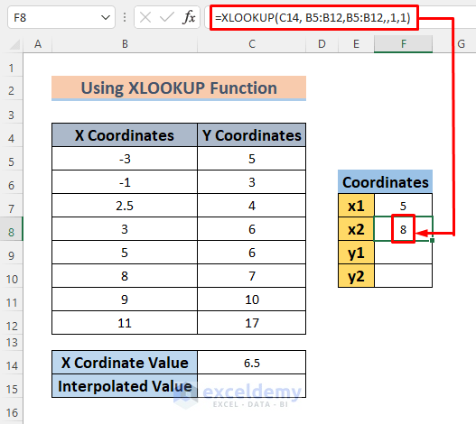
- Use the following formula in cell F8.
=XLOOKUP(C14, B5:B12,B5:B12,,1,1)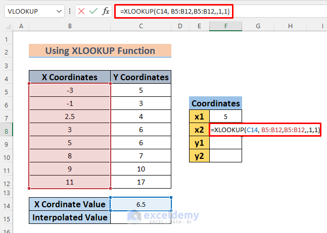
- Hit the Enter key and you will see a value above 6 in cell F8.
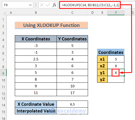
- Use the following formula in cell F9.
=XLOOKUP(C14, B5:B12,C5:C12,,-1,1)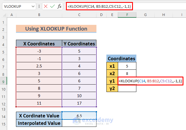
- Hit Enter.
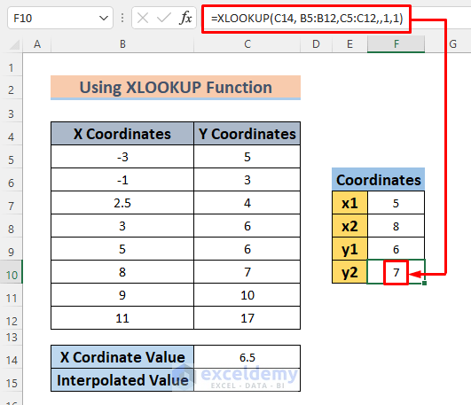
- Use this formula in cell F10.
=XLOOKUP(C14, B5:B12,C5:C12,,1,1)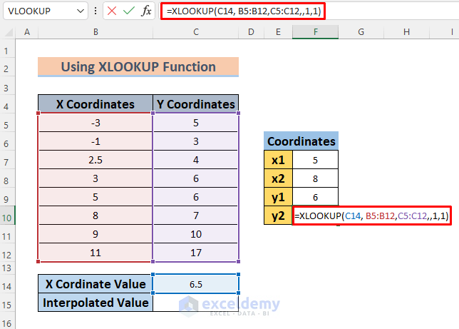
- Hit Enter and you will see the Y Coordinate that corresponds to X2.
- Select cell C15 and use the formula given below.
=FORECAST(C14,F9:F10,F7:F8)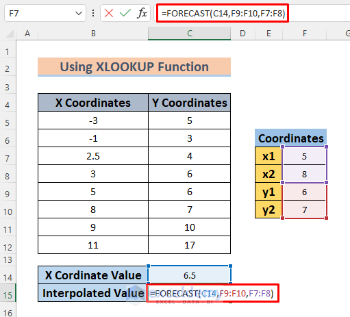
- Press the Enter key to see the interpolated value in cell C15.
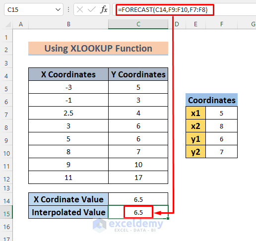
Note that the value is different since the FORECAST here has only two values to use as the baseline.
Method 3 – Inserting INDEX-MATCH with the FORECAST Function to Interpolate Between two Values
We want to interpolate the x-value 6 in B9:C10.
Steps:
- Modify the dataset to place the coordinates.
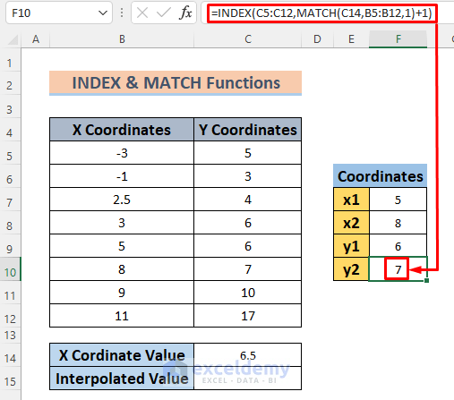
- Use the following formula in cell F7.
=INDEX(B5:B12,MATCH(C14,B5:B12,1))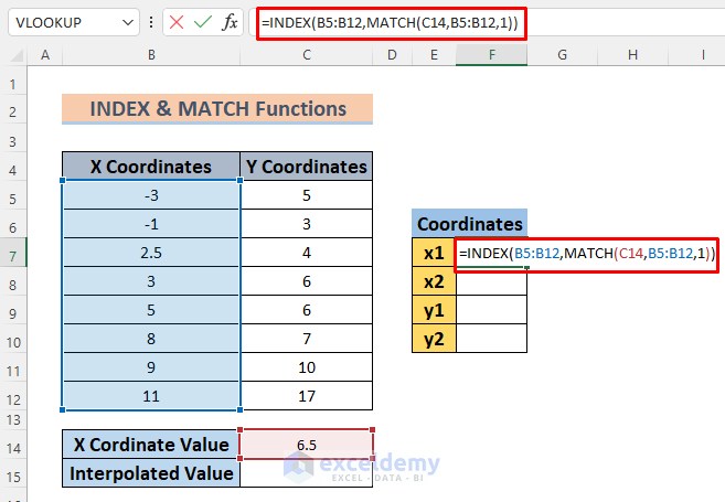
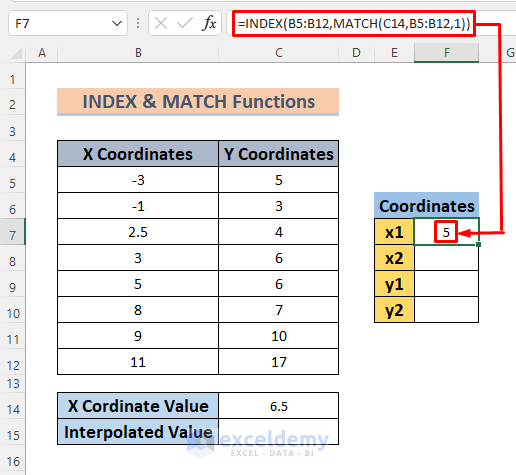
The MATCH function returns the position of the cell value of C14 in the range B5:B12. And then the INDEX function returns the value of that position in B5:B12. Thus, it returned x1.
A similar formula is used to determine x2, y1, and y2.
- Hit Enter to see the result in cell F7.
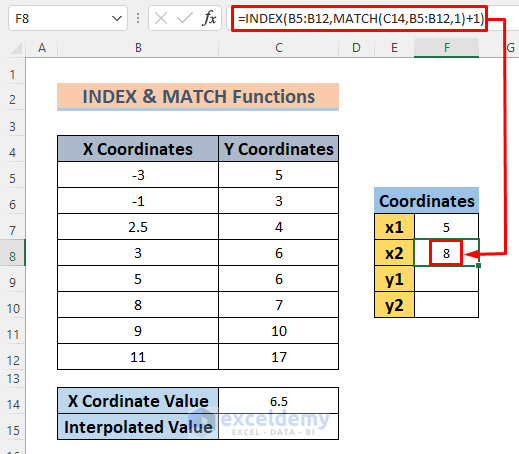
- Use the following formula in cell F8.
=INDEX(B5:B12,MATCH(C14,B5:B12,1)+1)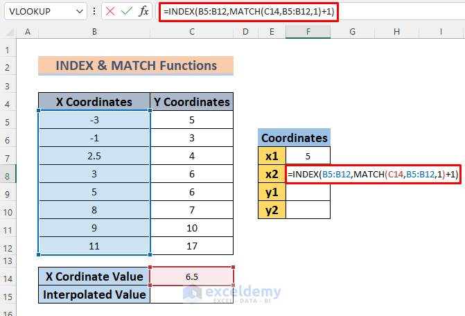
- Hit the Enter key, and you will see the next value above 6 in cell F8.
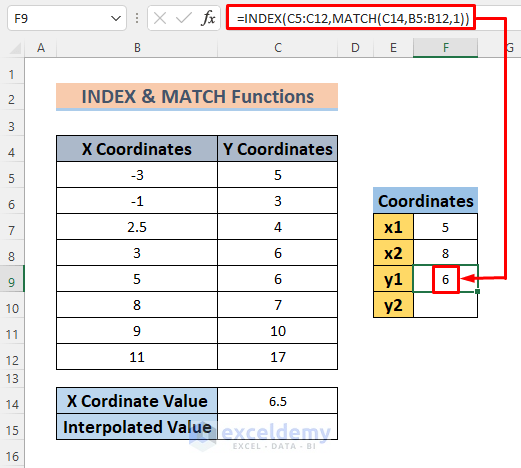
- Use the following formula in cell F9.
=INDEX(C5:C12,MATCH(C14,B5:B12,1))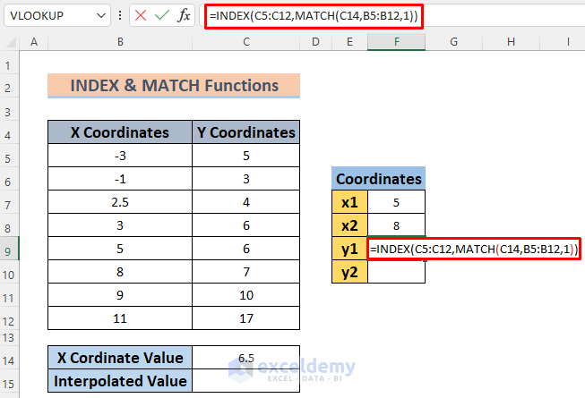
- Hit Enter. This returns the Y1 value that corresponds to X1.
- Use the following formula in cell F10.
=INDEX(C5:C12,MATCH(C14,B5:B12,1)+1)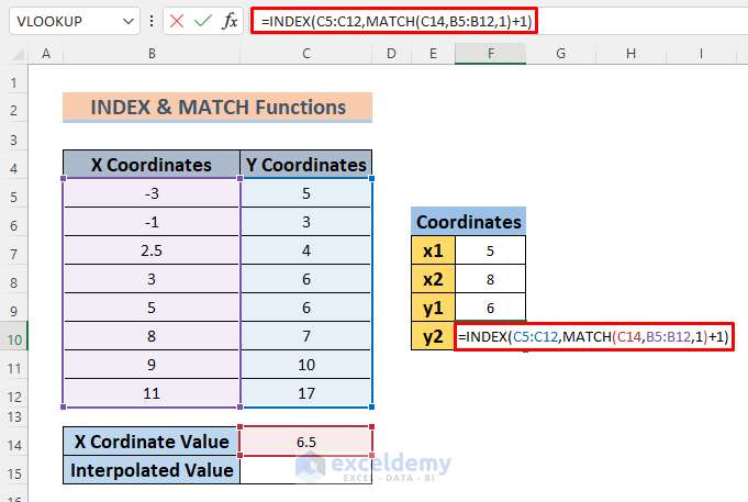
- Hit Enter.
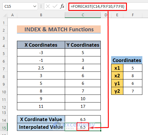
- Select cell C15 and insert the formula given below.
=FORECAST(C14,F9:F10,F7:F8)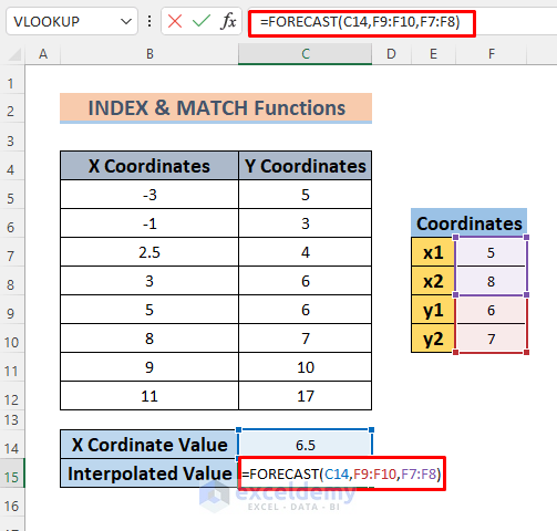
- Press the Enter key to see the interpolated value in cell C15.
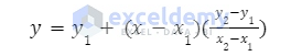
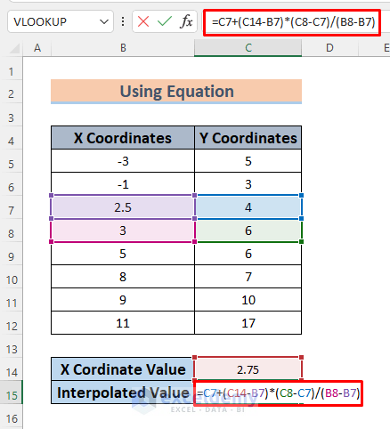
Method 4 – Interpolating Between Two Values by Applying a Mathematical Formula
The interpolation formula is given below. It uses an equation of a straight line.
Steps:
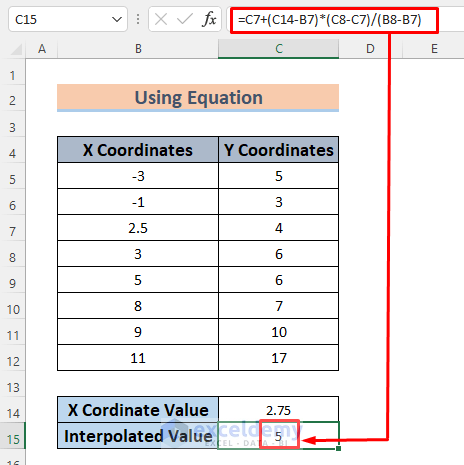
- Use the following formula in cell C15.
=C7+(C14-B7)*(C8-C7)/(B8-B7)We want to find the interpolated value when the X Coordinate is 2.75. For this reason, we chose the first available X Coordinates smaller or greater than 2.75 and their corresponding Y Coordinates in this dataset.
- Hit Enter to see the interpolated value in cell C15.
Read More: How to Interpolate in Excel Graph
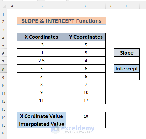
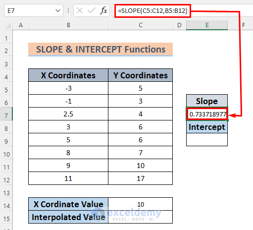
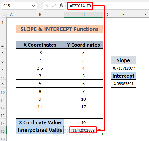
Method 5 – Interpolating between Two Values by Joining SLOPE and INTERCEPT Functions
We want to interpolate for X is 10.
Steps:
- Insert a few cells to store the slope.
- Insert the following formula in cell E7:
=SLOPE(C5:C12,B5:B12)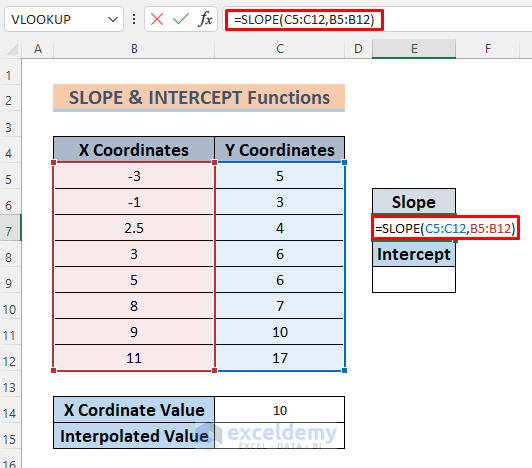
The SLOPE function returns the slope/gradient of the linear regression line which is made by the points formed by given X and Y Coordinates.
- Hit Enter.
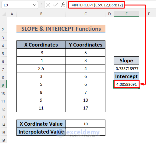
- Use the following formula in cell E9 to find the Y-intercept.
=INTERCEPT(C5:C12,B5:B12)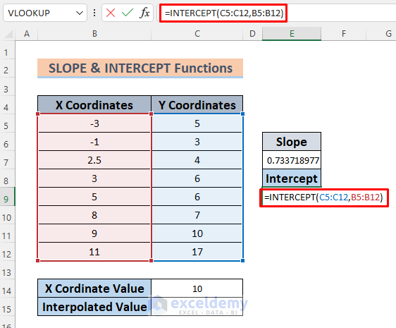
The INTERCEPT function returns the Y-intercept of the linear regression line which is made by the points formed by given X and Y Coordinates.
- Hit Enter to see the output in cell E9.
- Insert this formula in cell C15.
=E7*C14+E9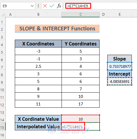
The formula is a basic straight-line formula, y=mx+c, where m is the slope and c is the intercept.
- Hit Enter to see the interpolated value in cell C15.
- Technically, you could combine all the functions to remove the need for helper cells.
Read More: How to Interpolate Missing Data in Excel
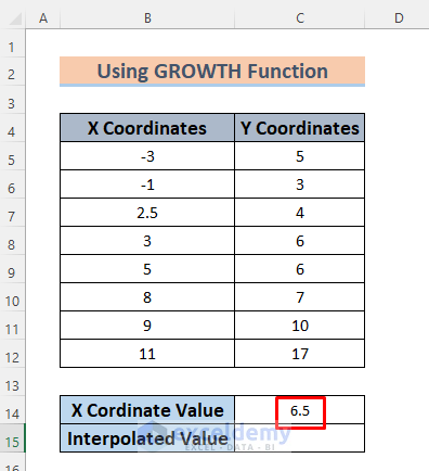
Method 6 – Using the Excel GROWTH Function for Nonlinear Interpolation
Our dataset has a non-linear relation between Y and X Coordinates.
Steps:
- We want to interpolate a value between 5 and 8. Let it be 6.5.
- Use the following formula in cell C15.
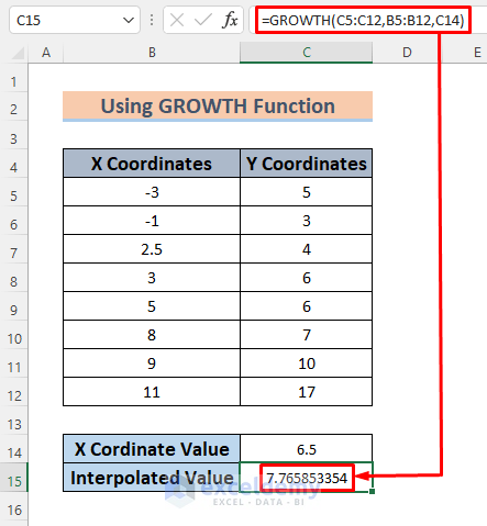
=GROWTH(C5:C12,B5:B12,C14)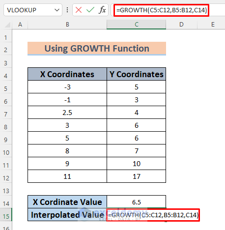
The GROWTH function returns the interpolated data by predicting the exponential growth of the X and Y Coordinates.
- Hit Enter and you will see the interpolated value in cell C15.
Download the Practice Workbook
Related Articles
- How to Do Interpolation with GROWTH & TREND Functions in Excel
- How to Do Linear Interpolation in Excel
- How to Perform Bilinear Interpolation in Excel
- How to Use Non-Linear Interpolation in Excel
- How to Do VLOOKUP and Interpolate in Excel
- How to Do Linear Interpolation Excel VBA
<< Go Back to Excel Interpolation | Excel for Statistics | Learn Excel
Get FREE Advanced Excel Exercises with Solutions!
