Method-1 – Using the IFERROR, VLOOKUP, and AVERAGE Functions to Do VLOOKUP and Interpolate
Steps:
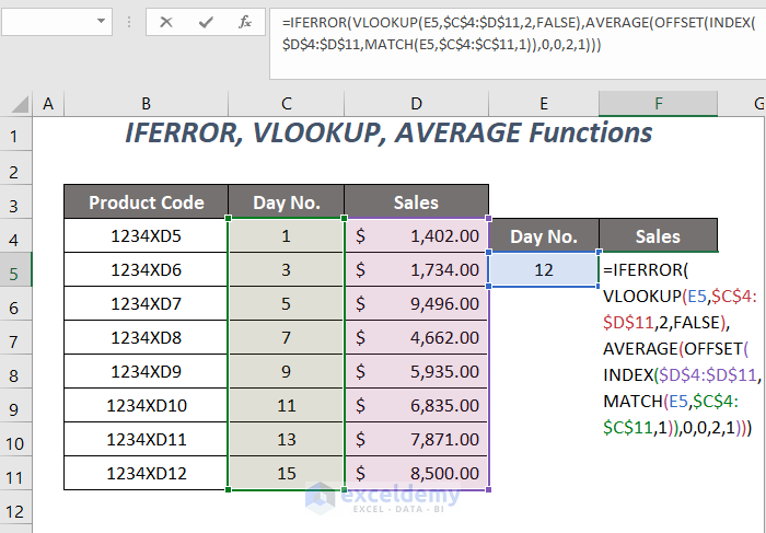
➤ Type the following formula in cell F5.
=IFERROR(VLOOKUP(E5,$C$4:$D$11,2,FALSE),AVERAGE(OFFSET(INDEX($D$4:$D$11,

MATCH(E5,$C$4:$C$11,1)),0,0,2,1)))
E5 is the look-up value, $C$4:$C$11 is the range of days numbers where we will look up value and $D$4:$D$11 is the range of the sales values.
- VLOOKUP(E5,$C$4:$D$11,2,FALSE) becomes
VLOOKUP(12,$C$4:$D$11,2, FALSE) → checks if 12 presents in the range $C$4:$C$11 and returns the corresponding sales values if it finds an exact match otherwise returns #N/A error.
Output → #N/A
- MATCH(E5,$C$4:$C$11,1) → gives the row index number for a day no. immediate less than 12 corresponding to the dataset; here, 1 is for finding the closest small value of 12.
Output → 6
- INDEX($D$4:$D$11,MATCH(E5,$C$4:$C$11,1)) becomes
INDEX($D$4:$D$11,6) → returns the cell reference number according to the row index number 6 from the range $D$4:$D$11.
Output → $D$9
- OFFSET(INDEX($D$4:$D$11,MATCH(E5,$C$4:$C$11,1)),0,0,2,1) becomes
OFFSET($D$9,0,0,2,1) → extracts a range with a height 2 starting from the cell $D$9.
Output → $D$9:$D$10
- AVERAGE(OFFSET(INDEX($D$4:$D$11,MATCH(E5,$C$4:$C$11,1)),0,0,2,1))) becomes
AVERAGE($D$9:$D$10) → returns the average of the values of this range
Output → 7353
- IFERROR(VLOOKUP(E5,$C$4:$D$11,2,FALSE),AVERAGE(OFFSET(INDEX($D$4:$D$11,MATCH(E5,$C$4:$C$11,1)),0,0,2,1))) becomes
IFERROR(#N/A,7353) → for errors, return the second argument 7353.
Output → $7,353.00
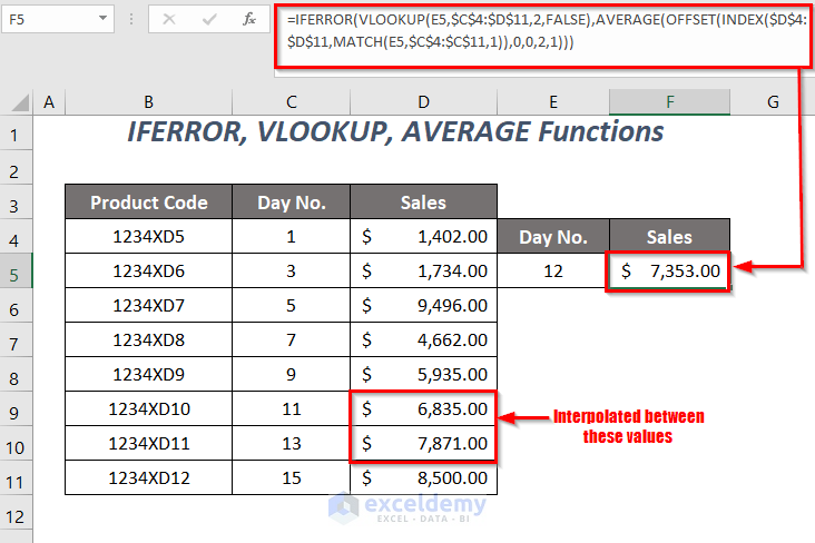
➤ Press ENTER.
You will get 7,353.00 for day 12, which is the interpolation of the sales values between days 11 and 13.
Method-2 – Combination of IF, ISNA, VLOOKUP, AVERAGE, and MINIFS Functions to Do VLOOKUP and Interpolate
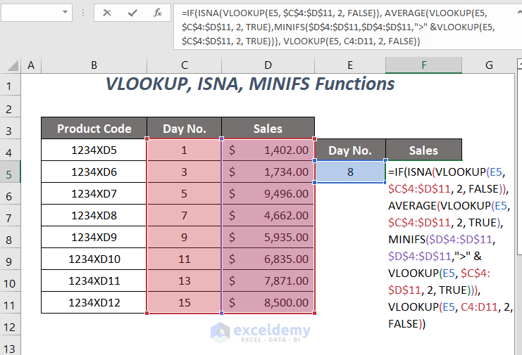
➤ Type the following formula in cell F5.
=IF(ISNA(VLOOKUP(E5, $C$4:$D$11, 2, FALSE)), AVERAGE(VLOOKUP(E5, $C$4:$D$11, 2, TRUE),MINIFS($D$4:$D$11,$D$4:$D$11,">" &VLOOKUP(E5, $C$4:$D$11, 2, TRUE))), VLOOKUP(E5, C4:D11, 2, FALSE))E5 is the look-up value, $C$4:$C$11 is the range of days numbers where we will look up value, and $D$4:$D$11 is the range of the sales values.
- VLOOKUP(E5, $C$4:$D$11, 2, FALSE) becomes
VLOOKUP(8,$C$4:$D$11,2, FALSE) → checks if 8 presents in the range $C$4:$C$11 and returns the corresponding sales values if it finds an exact match otherwise returns #N/A error.
Output → #N/A
- ISNA(VLOOKUP(E5, $C$4:$D$11, 2, FALSE)) becomes
ISNA(#N/A) → returns TRUE for #N/A error otherwise FALSE.
Output → TRUE
- VLOOKUP(E5, $C$4:$D$11, 2, TRUE) → finds an approximate match smallest near value presents in the range like for day 8, it will give the sales value for day 7
Output → 4662
- MINIFS($D$4:$D$11,$D$4:$D$11,”>” &VLOOKUP(E5, $C$4:$D$11, 2, TRUE) ) becomes
MINIFS($D$4:$D$11,$D$4:$D$11,”>” &4662) → MINIFS($D$4:$D$11,$D$4:$D$11,”>4662″) → returns the minimum value from the range $D$4:$D$11 based on the criteria that the values greater than 4662 in this range
Output → 5935
- AVERAGE(VLOOKUP(E5, $C$4:$D$11, 2, TRUE),MINIFS($D$4:$D$11,$D$4:$D$11,”>” &VLOOKUP(E5, $C$4:$D$11, 2, TRUE))) becomes
AVERAGE(4662, 5935) → returns the average of these values
Output → 5298.5
- IF(ISNA(VLOOKUP(E5, $C$4:$D$11, 2, FALSE)), AVERAGE(VLOOKUP(E5, $C$4:$D$11, 2, TRUE),MINIFS($D$4:$D$11,$D$4:$D$11,”>” &VLOOKUP(E5, $C$4:$D$11, 2, TRUE))), VLOOKUP(E5, C4:D11, 2, FALSE)) becomes
IF(TRUE, 5298.5, #N/A) → returns 5298.5 for TRUE otherwise #N/A
Output → $5,298.50
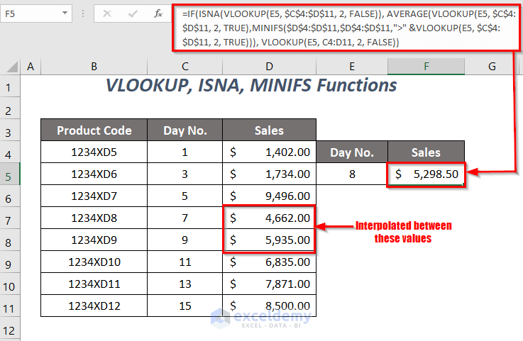
After pressing ENTER, you will get the sales value of $5,298.50 for day 8 by looking up the values in the range and interpolating between the sales values of days 7 and 9.
Method-3 – Using the Combination of the IF, ISNA, VLOOKUP, AVERAGE, INDEX, and MATCH Functions
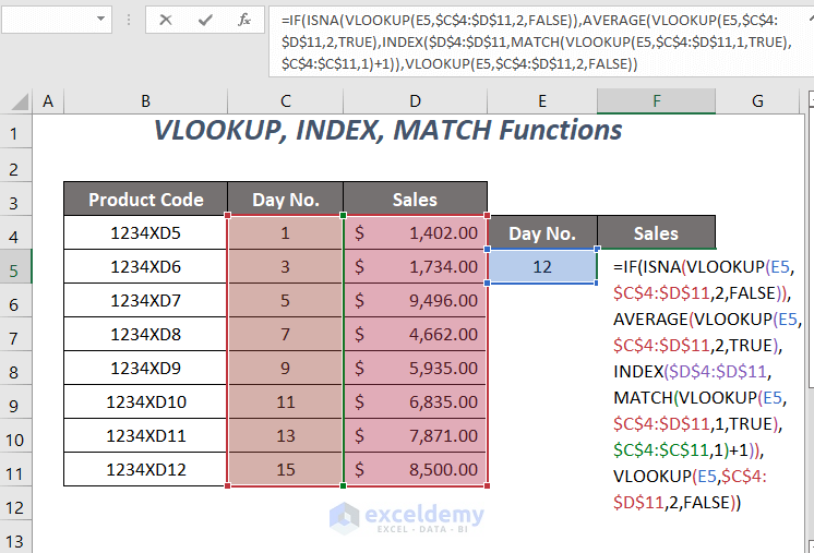
➤ Type the following formula in cell F5.
=IF(ISNA(VLOOKUP(E5,$C$4:$D$11,2,FALSE)),AVERAGE(VLOOKUP(E5,$C$4:$D$11,2,TRUE),INDEX($D$4:$D$11,MATCH(VLOOKUP(E5,$C$4:$D$11,1,TRUE),$C$4:$C$11,1)+1)),

VLOOKUP(E5,$C$4:$D$11,2,FALSE))
E5 is the look-up value, $C$4:$C$11 is the range of days numbers where we will look up value, and $D$4:$D$11 is the range of the sales values.
- VLOOKUP(E5, $C$4:$D$11, 2, FALSE) becomes
VLOOKUP(12,$C$4:$D$11,2, FALSE) → checks if 12 presents in the range $C$4:$C$11 and returns the corresponding sales values if it finds an exact match otherwise returns #N/A error.
Output → #N/A
- ISNA(VLOOKUP(E5, $C$4:$D$11, 2, FALSE)) becomes
ISNA(#N/A) → returns TRUE for #N/A error otherwise FALSE.
Output → TRUE
- VLOOKUP(E5, $C$4:$D$11, 2, TRUE) → finds an approximate match smallest near value presents in the range like for day, 12 it will give the sales value for day 11
Output → 6835
- VLOOKUP(E5,$C$4:$D$11,1,TRUE)
Output → 11
- MATCH(VLOOKUP(E5,$C$4:$D$11,1,TRUE),$C$4:$C$11,1) becomes
MATCH(11,$C$4:$C$11,1) → gives the row index number for a day no. immediate less than 12 corresponding to the dataset and here 1 is for finding the closest small value of 12.
Output → 6
- MATCH(VLOOKUP(E5,$C$4:$D$11,1,TRUE),$C$4:$C$11,1)+1 becomes
6+1 → adds up 1 for getting the row index number of the day no. 13
Output → 7
- INDEX($D$4:$D$11,MATCH(VLOOKUP(E5,$C$4:$D$11,1,TRUE),$C$4:$C$11,1)+1)) becomes
INDEX($D$4:$D$11,7) → returns the cell reference number according to the row index number 7 from the range $D$4:$D$11.
Output → $D$10
- AVERAGE(VLOOKUP(E5,$C$4:$D$11,2,TRUE),INDEX($D$4:$D$11,MATCH(VLOOKUP(E5,$C$4:$D$11,1,TRUE),$C$4:$C$11,1)+1)) becomes
AVERAGE(6835,$D$10) → AVERAGE(6835,7871)
Output → 7353
- IF(ISNA(VLOOKUP(E5,$C$4:$D$11,2,FALSE)),AVERAGE(VLOOKUP(E5,$C$4:$D$11,2,TRUE),INDEX($D$4:$D$11,MATCH(VLOOKUP(E5,$C$4:$D$11,1,TRUE),$C$4:$C$11,1)+1)),VLOOKUP(E5,$C$4:$D$11,2,FALSE)) becomes
IF(TRUE, 7353, #N/A) → returns 7353 for TRUE otherwise #N/A
Output → $7,353.00
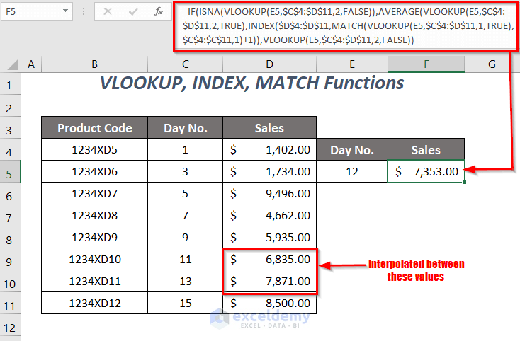
➤ Press ENTER.
You will get 7,353.00 for day 12, which is the interpolation of the sales values between days 11 and 13.
Method-4 – Do VLOOKUP and Interpolate in Excel Using the FORECAST, OFFSET, and MATCH Functions
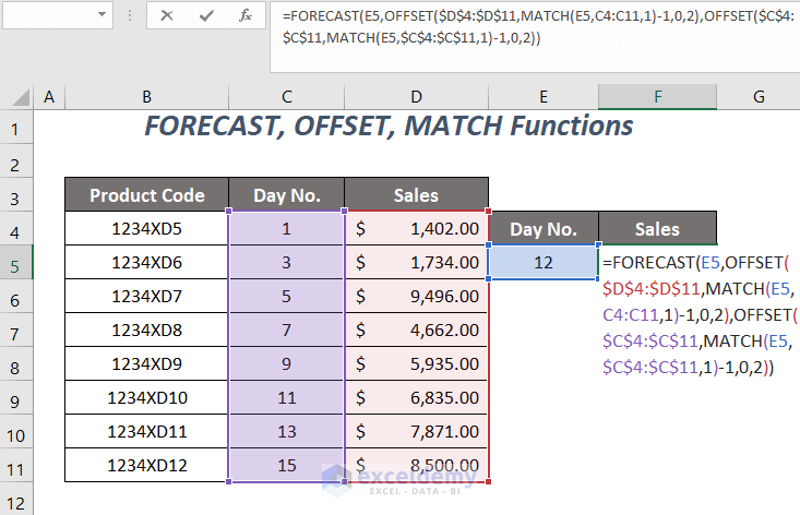
➤ Use the following formula in cell F5.
=FORECAST(E5,OFFSET($D$4:$D$11,MATCH(E5,C4:C11,1)-1,0,2),OFFSET($C$4:$C$11,

MATCH(E5,$C$4:$C$11,1)-1,0,2))
E5 is the look-up value, $C$4:$C$11 is the range of days numbers where we will look up value, and $D$4:$D$11 is the range of the sales values.
- MATCH(E5,C4:C11,1) becomes
MATCH(12, C4:C11,1) → gives the row index number for a day no. immediate less than 12 corresponding to the dataset, and here 1 is for finding the closest small value of 12.
Output → 6
- MATCH(E5,C4:C11,1)-1 becomes
6-1 → 5
- OFFSET($D$4:$D$11,MATCH(E5,C4:C11,1)-1,0,2) becomes
OFFSET($D$4:$D$11,5,0,2) → the new reference is set to the cell $D$9 after moving 5 rows downwards from $D$4 and then extracts a range of height 2 from the cell $D$9
Output → {6835; 7871}
- OFFSET($C$4:$C$11,MATCH(E5,$C$4:$C$11,1)-1,0,2) becomes
OFFSET($C$4:$C$11,5) → the new reference is set to the cell $C$9 after moving 5 rows downwards from $C$4 and then extracts a range of height 2 from the cell $C$9
Output → {11; 13}
- FORECAST(E5,OFFSET($D$4:$D$11,MATCH(E5,C4:C11,1)-1,0,2),OFFSET($C$4:$C$11,MATCH(E5,$C$4:$C$11,1)-1,0,2)) becomes
FORECAST(12,{6835; 7871},{11; 13}) → gives the value after doing interpolation
Output → $7,353.00
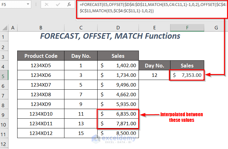
After pressing ENTER, you will get the sales value of $7,353.50 for day 12 by looking up the values in the range and interpolating between the sales values of days 11 and 13.
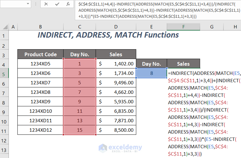
Method-5 – Using the Combination of INDIRECT, ADDRESS, and MATCH Functions
➤ Apply the following formula in cell F5.
=INDIRECT(ADDRESS(MATCH(E5,$C$4:$C$11,1)+3,4))+(INDIRECT(ADDRESS(MATCH(E5,$C$4:$C$11,1)+4,4))-INDIRECT(ADDRESS(MATCH(E5,$C$4:$C$11,1)+3,4)))/

(INDIRECT(ADDRESS(MATCH(E5,$C$4:$C$11,1)+4,3))-INDIRECT(ADDRESS(MATCH(E5,$C$4:$C$11,1)+3,3)))*

(E5-INDIRECT(ADDRESS(MATCH(E5,$C$4:$C$11,1)+3,3)))
E5 is the look-up value, $C$4:$C$11 is the range of days numbers where we will look up value, and $D$4:$D$11 is the range of the sales values.
MATCH(E5,$C$4:$C$11,1)→ gives the row index number for a day no. immediate less than 8 corresponding to the dataset and here 1 is for finding the closest small value of 8.
Output → 4
MATCH(E5,$C$4:$C$11,1)+3becomes
4+3 → 3 is added here because our dataset has started after Row 3
Output → 7
ADDRESS(MATCH(E5,$C$4:$C$11,1)+3,4)becomes
ADDRESS(7,4)→ returns the cell reference for a cell with row 7 and column 4
Output → “$D$7”
INDIRECT(ADDRESS(MATCH(E5,$C$4:$C$11,1)+3,4))becomes
INDIRECT(“$D$7”)→ returns the value of this cell
Output → 4662
MATCH(E5,$C$4:$C$11,1)+4becomes
4+4 → 3 (3+1=4) is added here because our dataset has started after Row 3, and another 1 is for having the value for day 9
Output → 8
INDIRECT(ADDRESS(MATCH(E5,$C$4:$C$11,1)+4,4))becomes
INDIRECT(ADDRESS(8,4))→INDIRECT(“$D$8”)
Output → 5935
INDIRECT(ADDRESS(MATCH(E5,$C$4:$C$11,1)+4,4))-INDIRECT(ADDRESS(MATCH(E5,$C$4:$C$11,1)+3,4))becomes
5935-4662
Output → 1273
INDIRECT(ADDRESS(MATCH(E5,$C$4:$C$11,1)+4,3)becomes
INDIRECT(ADDRESS(8,3)) → INDIRECT(“$C$8”)
Output → 9
INDIRECT(ADDRESS(MATCH(E5,$C$4:$C$11,1)+3,3)becomes
INDIRECT(ADDRESS(7,3))→INDIRECT(“$C$7”)
Output → 7
(INDIRECT(ADDRESS(MATCH(E5,$C$4:$C$11,1)+4,3))-INDIRECT(ADDRESS(MATCH(E5,$C$4:$C$11,1)+3,3)))becomes
9-7
Output → 2
E5-INDIRECT(ADDRESS(MATCH(E5,$C$4:$C$11,1)+3,3))becomes
8-7
Output → 1
INDIRECT(ADDRESS(MATCH(E5,$C$4:$C$11,1)+3,4))+(INDIRECT(ADDRESS(MATCH(E5,$C$4:$C$11,1)+4,4))-INDIRECT(ADDRESS(MATCH(E5,$C$4:$C$11,1)+3,4)))/(INDIRECT(ADDRESS(MATCH(E5,$C$4:$C$11,1)+4,3))-INDIRECT(ADDRESS(MATCH(E5,$C$4:$C$11,1)+3,3)))*(E5-INDIRECT(ADDRESS(MATCH(E5,$C$4:$C$11,1)+3,3)))becomes
4662+((1273)/(2))*1
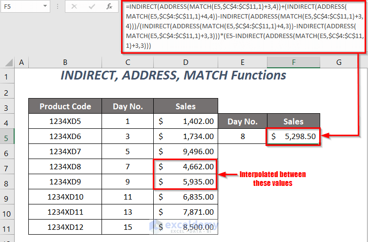
Output → $5,298.50
➤ Press ENTER.
You will get the sales value of $5,298.50 for day 8 by looking up the values in the range and interpolating between the sales values of days 7 and 9.
Method-6 – Using VBA Code to Do VLOOKUP and Interpolate in Excel
Steps:
➤ Go to the Developer Tab >> Visual Basic Option.
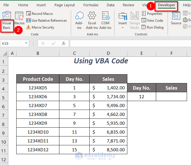
The Visual Basic Editor will open up.
➤ Go to the Insert Tab >> Module Option.
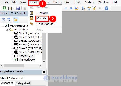
A Module will be created.
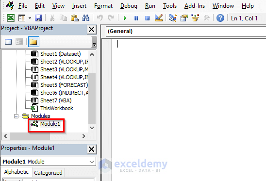
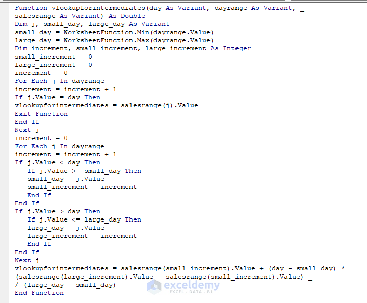
➤ Write the following code
Function vlookupforintermediates(day As Variant, dayrange As Variant, _
salesrange As Variant) As Double

Dim j, small_day, large_day As Variant
small_day = WorksheetFunction.Min(dayrange.Value)
large_day = WorksheetFunction.Max(dayrange.Value)
Dim increment, small_increment, large_increment As Integer
small_increment = 0
large_increment = 0
increment = 0

For Each j In dayrange
increment = increment + 1
If j.Value = day Then
vlookupforintermediates = salesrange(j).Value
Exit Function
End If
Next j

increment = 0

For Each j In dayrange
increment = increment + 1
If j.Value < day Then
   If j.Value >= small_day Then
   small_day = j.Value
   small_increment = increment
   End If
End If
If j.Value > day Then
   If j.Value <= large_day Then
   large_day = j.Value
   large_increment = increment
   End If
End If
Next j

vlookupforintermediates = salesrange(small_increment).Value + (day - small_day) * _
(salesrange(large_increment).Value - salesrange(small_increment).Value) _
/ (large_day - small_day)

End Function
We created a function with the name vlookupforintermediates, and the variables under this function as inputs are day, dayrange, and salesrange all of them are declared as Variant. We declared j, small_day, and large_day as Variant and increment, small_increment, and large_increment as Integer.
Using the MIN and MAX functions small_day and large_day are assigned to the smallest and largest days.
The first FOR loop will return the sales values for any day which is present in the day’s ranges and the second FOR loop with the IF-Then statement will store value to the small_increment and large_increment variables.
Using the formula for calculating interpolation, this function will return our desired value.
After saving the code, you have to return to the main sheet.
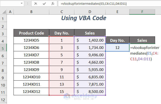
➤ Use the following formula in cell F5.
=vlookupforintermediates(E5,C4:C11,D4:D11)The vlookupforintermediates is the created function name, E5 is the day, C4:C11 is the dayrange, and D4:D11 is the salesrange.
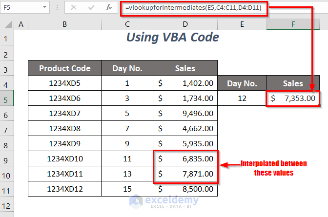
➤ Press ENTER.
You will get the sales value of $7,353.00 for the specific day no. 12.
Download Workbook
Related Articles
- How to Do Linear Interpolation in Excel
- How to Interpolate Missing Data in Excel
- How to Do Interpolation with GROWTH & TREND Functions in Excel
- How to Interpolate Between Two Values in Excel
- How to Perform Bilinear Interpolation in Excel
- How to Use Non Linear Interpolation in Excel
<< Go Back to Excel Interpolation | Excel for Statistics | Learn Excel
Get FREE Advanced Excel Exercises with Solutions!
