Method 1 – Use of Linear Trend Method
Using linear interpolation, we can estimate missing data using a straight line that connects two known values.
Formula:
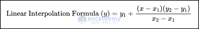
(x1, y1) = The First coordinate of the interpolation process.
(x2,y2) = Second point of the interpolation process.
x = Known value.
y =Unknown value.
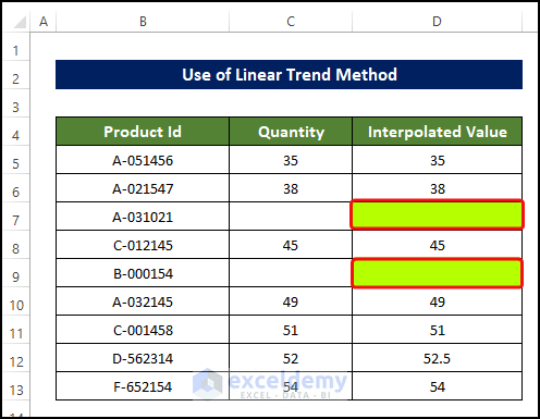
The dataset that we are going to use has this linear pattern, although it has some of its data missing, as seen in the image. The missing data point can be demonstrated by the discontinuities in the line.
If your dataset follows this pattern, then you can use the below method to extract the missing value.
Steps
- We have the below dataset where data is missing in cells C7 and C9.
- Using the surrounding values, we need to estimate the quantity values in those cells.
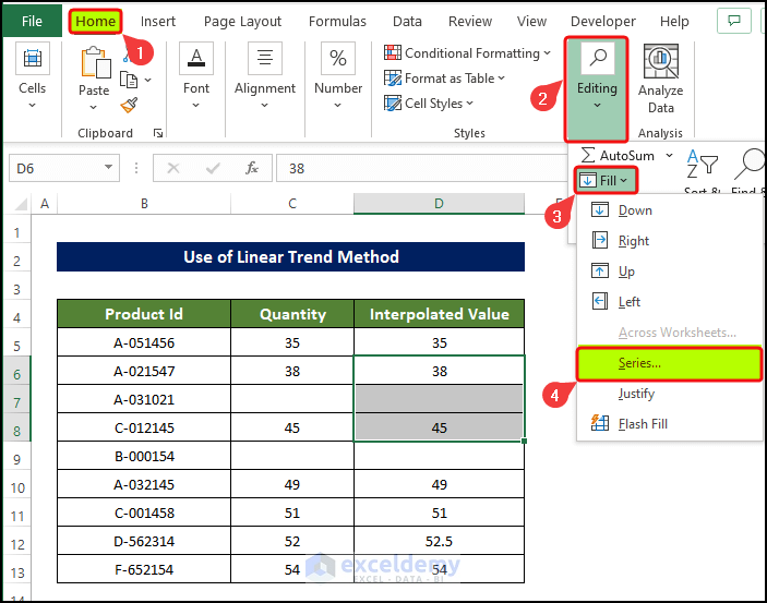
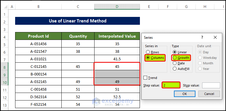
- Select the range of cells D6:D8, and go to the Home tab > Editing.
- Go to Fill > Series.
- In the Series window, click on the Columns in the Series in option and select Linear in the Type option.
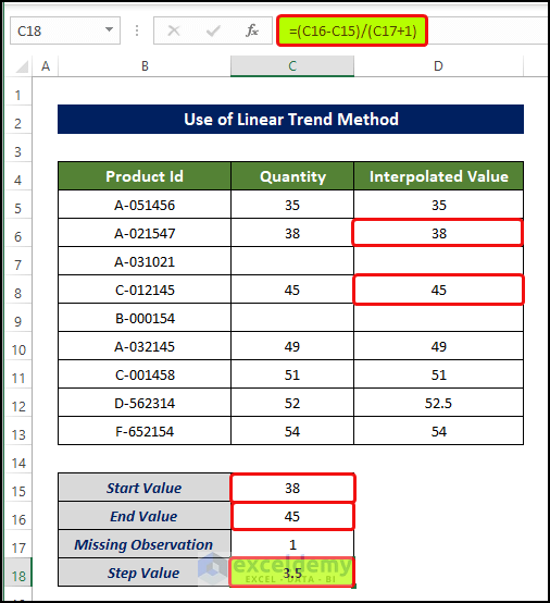
- You can see that the Step values are now set to 2.5 by default. You can edit these values as per needs.
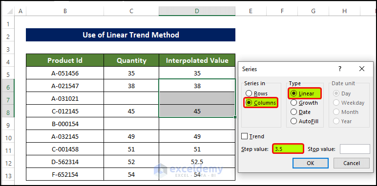
- You can also calculate the step value using the following formula in the cell C18:
=(C16-C15)/(C17+1)
- Repeat the same process for cell D9.
- In order to get the missing value of the D9 cell, select the range of cells D8:D10, and go to the Home tab > Editing.
- Go to Fill > Series.
- In the Series window, click on the Columns in the Series in option and select Linear in the Type option.
- You can see that the Step values are now set to 2.5 by default.
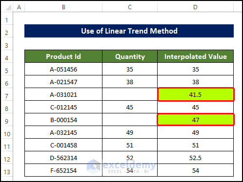
- Click OK.
- The cell with the missing values now has the values retrieved by using the Linear Trend.
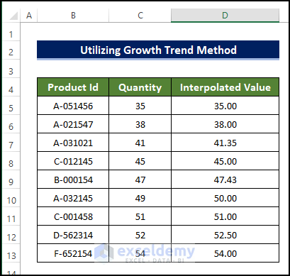
Method 2 – Utilizing Growth Trend Method
When predicting future growth based on past data, growth trend interpolation in Excel can be useful. Linear growth suggests a constant increase throughout time, resulting in a straight path on a graph. This means that the annual percentage increase is decreasing slightly with each passing year.
Steps
- In the dataset, data is missing in cells C7 and C9.
- Using the surrounding values, we need to estimate the quantity values in those cells.
- Select the range of cells D6:D8 and go to the Home tab > Editing.
- Go to Fill > Series.
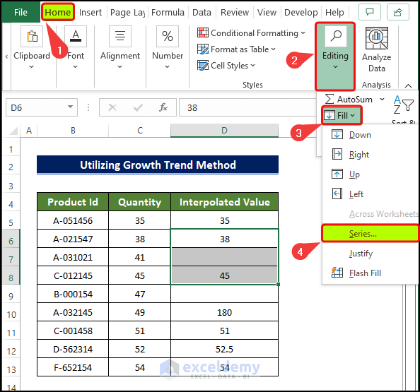
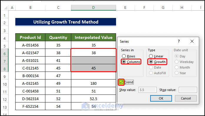
- In the Series window, click on the Columns in the Series in option and select Growth in the Type option.
- Tick the Trend check box and click OK.
- Repeat the same process for the second missing value in cell D9.
- Select the range of cells D8:D10 and go to the Home tab > Editing.
- Go to Fill > Series.
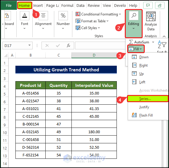
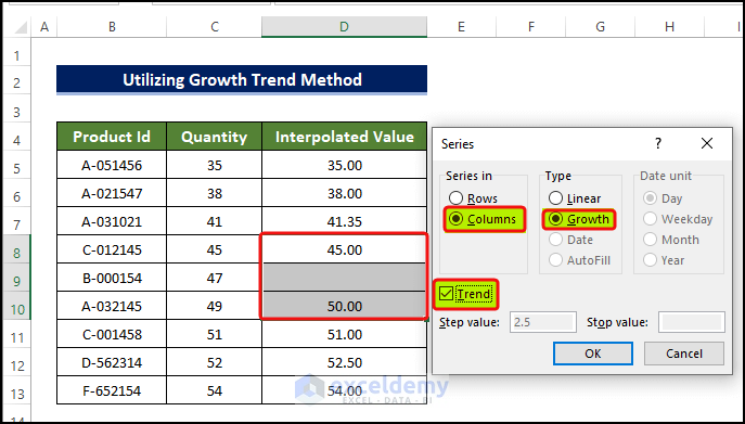
- In the Series window, click on the Columns in the Series in option and select Growth in the Type option.
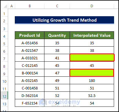
- Tick the Trend check box and click OK.
- The cells D9 and D7 now have the missing value.
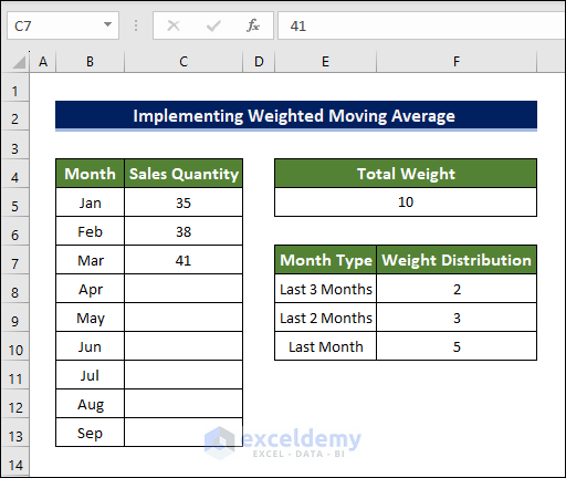
Method 3 – Implementing Weighted Moving Average Formula
We have another sample dataset with two columns, Named Month and Sales Quantity, with range B4:C13 like the following image. We are considering 10 as the total weight (Wt) and distributing the Wt among the previous month in such a way that recent data gets more weight. We have data only for January, February, and March. We will interpolate the Sales Quantity for the rest of the months.
Definition:
The weighted moving average (WMA) is a useful metric that gives more weight to the latest data points and less weight to datasets from a long time ago.
Formula:
![]()
A1, A2, A3, A4 ….., is the data point of the datasets.
W1, W2, W3, W4…… are the weight assigned to each data point.
Wt is the summation of all weights.
Let’s apply the above theory to our dataset.
Follow these steps:
Step 1: Select cell C8 => Insert the given formula.
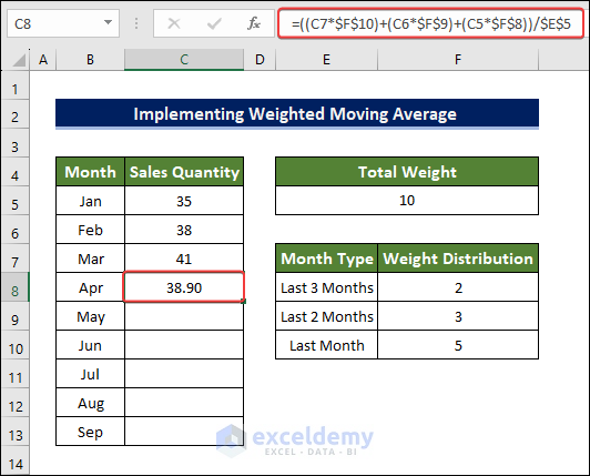
=((C7*$F$10)+(C6*$F$9)+(C5*$F$8))/$E$5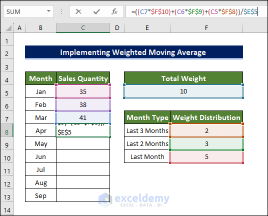
Step 2: Hit Enter to see the result.
Step 3: Hover over the cursor to the bottom right corner of cell C8 to see the Fill Handle icon.
![]()
Step 4: Drag the Fill Handle icon to cell C13 to copy the formula.
![]()
Method 4 – Using Simple Moving Average Formula
Definition:
Simple moving averages compute the average of a price range over a given number of periods.
Formula:
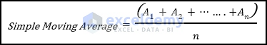
A1, A2, A3, A4……An is the data point of the datasets.
N = Denotes the number of data points.
A simple moving average is a measurement tool that can help predict if an asset price will maintain or if it falls into reverse bull even in a bear trend. We will consider the dataset of the first two methods and use the AVERAGE and IF function alongside the weighted moving average to estimate the missing value.
Steps
- Choose the span range. We chose span 3.
- Average the value, which will be done in a spanwise row.
- If we have a missing value in cell C7, the formula span of this cell would be E6:E8.
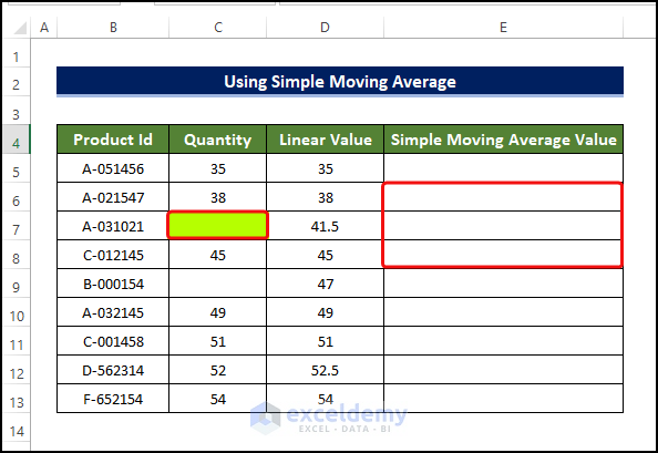
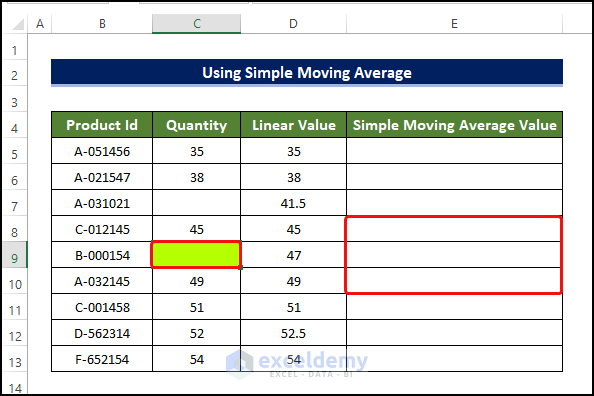
- If we have a missing value in cell C9, the formula span of this cell would be E8:E10.
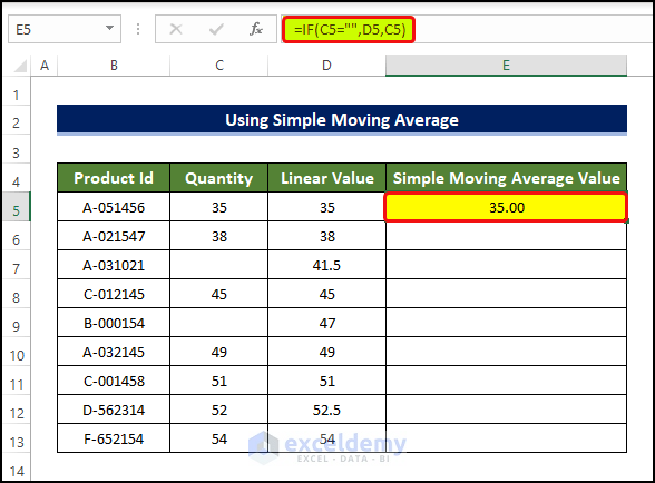
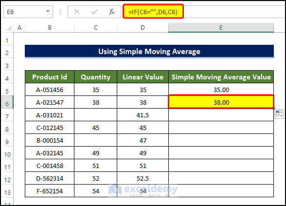
- Select cell E5 and enter the following formula:
=IF(C5="",D5,C5)
- Repeat the same formula in the cell E6 and enter the following formula:
=IF(C6="",D6,C6)
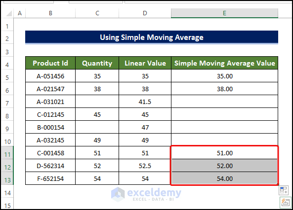
- Select cell E11 and enter the following formula:
=IF(C11="",D11,C11)

- Drag the Fill Handle to cell E13.
- Select cell E7 and enter the following formula:
=IF(C7="",AVERAGE(D5:D9),C7)
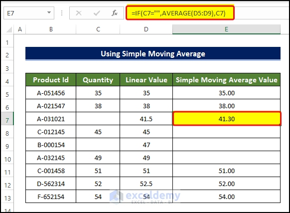
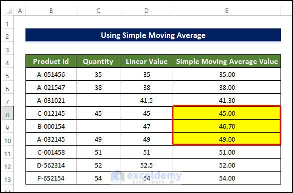
- Drag the Fill Handle to cell E10.
- This will fill the range of cell E8:E10 with a Simple Moving Average Value.
- Cell E9 now also has the missing value presented of cell C9.
Download Practice Workbook
Related Articles
- How to Do Linear Interpolation in Excel
- How to Do Interpolation with GROWTH & TREND Functions in Excel
- How to Do VLOOKUP and Interpolate in Excel
- How to Interpolate Between Two Values in Excel
- How to Perform Bilinear Interpolation in Excel
- How to Use Non Linear Interpolation in Excel
- How to Interpolate in Excel Graph
- How to Do Linear Interpolation Excel VBA
<< Go Back to Excel Interpolation | Excel for Statistics | Learn Excel
Get FREE Advanced Excel Exercises with Solutions!

How do you determine the value of the weight for method 3?
Hello CYNTHIA
Thanks for visiting our blogs and sharing your queries. You want to know how to initialize the weight in the method 3. When investigating your problem, we found that the dataset we previously used does not suit the weighted moving average formula. So, we have modified the article (method 3) for better understanding.
When implementing a weighted moving average formula, it is better to fix the total weight first and distribute the weights among durations. So, please go to method 3 of this article again. Hopefully, you will not have any doubts. Good luck!
Regards
Lutfor Rahman Shimanto
ExcelDemy