In this tutorial, we will explain how to do interpolation in Excel with GROWTH & TREND functions. In mathematics, interpolation is a statistical strategy for estimating an unknown value using related known variables. Microsoft Excel does not provide any direct function for interpolation. So, we use different functions to calculate a new value from known X and Y Values.
Interpolation with GROWTH & TREND Functions in Excel: 2 Methods
In this tutorial, we’ll apply the GROWTH & TREND functions to interpolate a new value from a dataset. Apart from this, we’ll go over another method that uses a trendline to interpolate a new value.
1. Do Interpolation in Excel with GROWTH Function
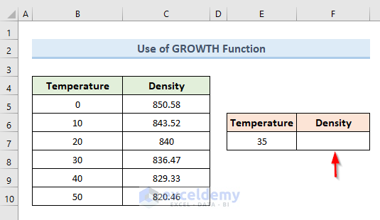
First and foremost, we will interpolate a new value from the following dataset using the GROWTH function. The following dataset consists of values of different temperatures with corresponding densities. Using these data, we want to estimate the density at a temperature of 35° Celsius.
Let’s see the steps to perform this action:
STEPS:
- To begin with, select cell F7.
- In addition, insert the following formula in that cell:
=GROWTH(C5:C10,B5:B10,E7,1)- Then, press Enter.
- Lastly, in cell F7 we get the value of density for the temperature of 35° celsius. We can see that the value of the density in cell F7 is 06 kg/m³.

2. Interpolation with TREND Function in Excel
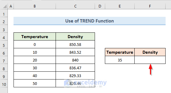
In the second method, we will use the TREND function to do interpolation in Excel. To illustrate this method, we will use the same dataset that we used in the previous method. Also, we will interpolate data to get the value of density for 35° celsius.
Just follow the steps below to execute this method.
STEPS:
- First, select cell F7.
- Next, type the following formula in that cell:
=TREND(C5:C10,B5:B10,E7,1)- After that, hit Enter.
- Finally, we can see the value of density for 35° celsius temperature in cell F7. The estimated value of density is 11 kg/m³.

NOTE:
If we notice, we will see that the values that we get using the GROWTH function and TREND function are different. We get the value of density of 831.06 kg/m³ when we use the GROWTH function and 831.11 kg/m³ when we use the TREND function. In terms of interpolation, the value that we get using the GROWTH function is more accurate than that we get using the TREND function.
How to Use Trendline in Excel to Do Nonlinear Interpolation in Excel
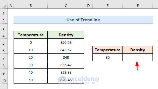
In this method, we will use neither the GROWTH function nor the TREND function to do interpolation in Excel. Rather, we will use a trendline to interpolate new values. While we are working with nonlinear data, we need to figure out the function’s behavior first. With the help of a trend line, we will develop an equation that matches our data. Then, using that equation, we will interpolate a new value.
To make you understand better, we will again interpolate the value of density for 35° celsius temperature.
Let’s take a look at the steps to perform this method.
STEPS:
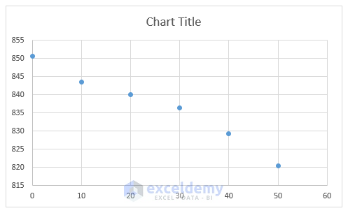
- Firstly, select the data range (B5:C10).
- Next, go to the Insert from the Charts section under the Insert tab and select the first scattered graph.
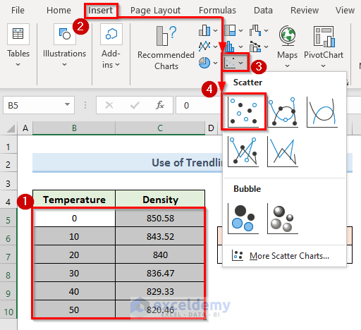
- So, we will get a graph like the following image.
- Then, click on the graph.
- After that, go to Add Chart Element > Trendline > Linear.
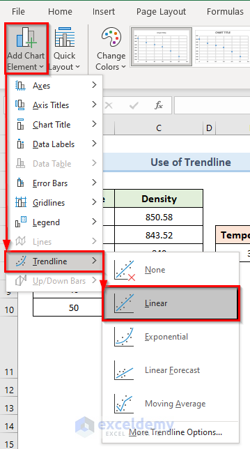
- The above action will return a trendline in the graph.
- Next, double-click on the trend line.
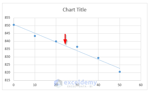
- Now, we can see a new sidebar named ‘Format Trendline’.
- Furthermore, scroll down and check the option ‘Display Equation on chart’.

- The above action shows the equation on the graph that matches best with the pattern of our data.

- After that, insert the equation in cell F7. Instead of x in the equation using the cell value of E7.
=-0.562*E7 + 850.78
- Press Enter.
- In the end, we get the value of density at 35° celsius temperature in cell F7.

Read More: How to Interpolate in Excel Graph
Download Practice Workbook
We can download the practice workbook from here.
Conclusion
In conclusion, this tutorial shows how to do interpolation in Excel using the GROWTH and TREND functions. Use the practice worksheet that comes with this article to put your skills to the test. If you have any questions, please leave a comment below. Our team will make every effort to react to you as quickly as possible. Keep an eye out for more inventive Microsoft Excel solutions in the future.
Related Articles
- How to Interpolate Missing Data in Excel
- How to Interpolate Between Two Values in Excel
- How to Do Linear Interpolation in Excel
- How to Do VLOOKUP and Interpolate in Excel
- How to Perform Bilinear Interpolation in Excel
- How to Use Non Linear Interpolation in Excel
- How to Do Linear Interpolation Excel VBA
<< Go Back to Excel Interpolation | Excel for Statistics | Learn Excel
Get FREE Advanced Excel Exercises with Solutions!
