Let’s say, you know the values of two known points A (x1,y1) and C (x2,y2) of a straight line and you want to determine the unknown value y from the point of B (x,y) when you also know the x. In that case, the mathematical equation is as follows:
y=y1+ (x-x1)*(y2-y1)/(x2-x1)
Linear Interpolation in Excel: 7 Methods
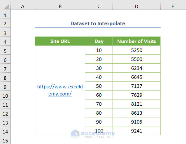
Let’s introduce the following dataset where the Number of Visits is given on the basis of the Day of a well-known Excel learning website. Now, you need to interpolate the Number of Visits for a specific Day.
Method 1 – Using the Equation of the Linear Interpolation
Suppose you want to find the Number of Visits for Day number 55.
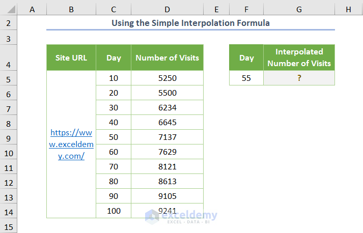
- Insert the following formula in the G5 cell:
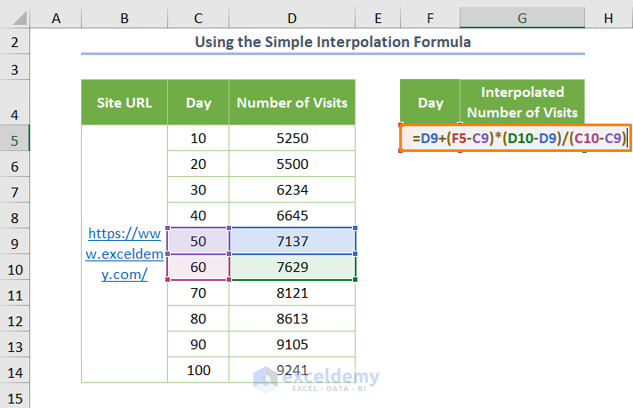
=D9+(F5-C9)*(D10-D9)/(C10-C9)
Here, D9 and D10 are the Number of Visits for Day numbers 50 and 60 respectively whereas C9 and C10 are the cells having the values of the corresponding Day.
But why do you need cells C9 and C10? Because you want to interpolate for Day 50 and it lies between those cells.
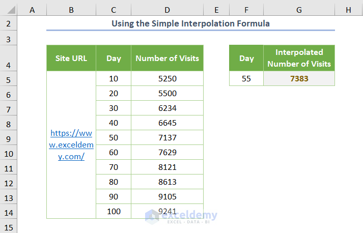
- After pressing Enter, you’ll get the interpolated Number of Visits is 7383.
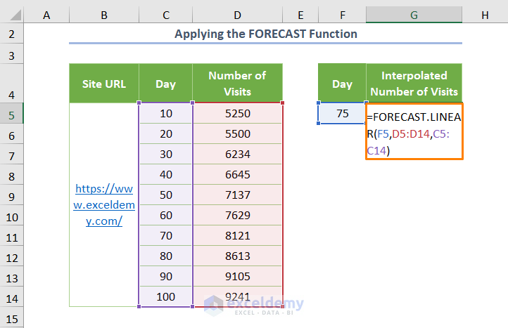
Method 2 – Applying the FORECAST Function to Do Linear Interpolation
- Here’s a function to determine the Number of Visits for Day 75:
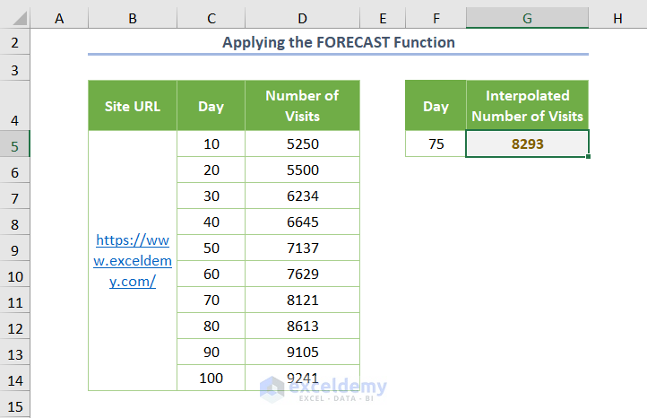
=FORECAST.LINEAR(F5,D5:D14,C5:C14)
F5 represents the value for which you want to interpolate, D5:D14 is the known_y’s argument which is mainly the dependent range of data (Number of Visits) and the C5:C14 is the known_x’s argument representing the independent range of data (Day).
- You’ll get the following output.
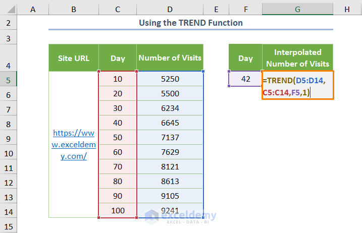
Method 3 – Using the TREND Function
Use the following formula:
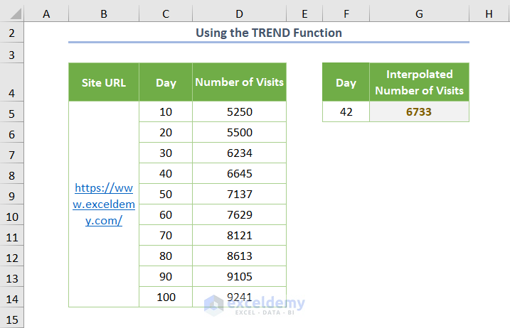
=TREND(D5:D14,C5:C14,F5,1)
Here, 1 is for defining the value of const is 0.
The output will look as follows.
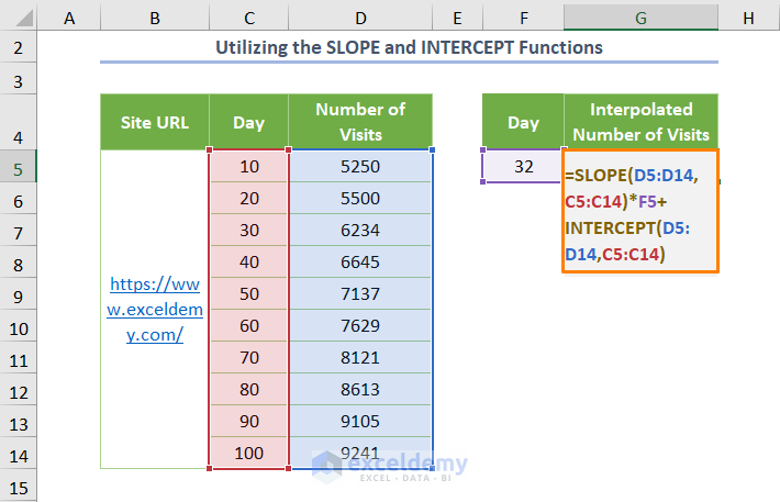
Method 4 – Utilizing the SLOPE and INTERCEPT Functions
You can also interpolate via the equation for the simple linear regression. That is Y = a + bX, where Y and X are the dependent and independent variables. Here, a is the intercept and b is the slope value.
- Use the following formula:
=SLOPE(D5:D14,C5:C14)*F5+INTERCEPT(D5:D14,C5:C14)
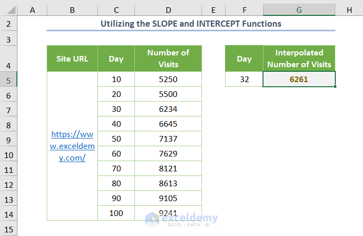
While computing the linear interpolation, you need to multiply the slope (as illustrated in the equation) with the independent variable (value of Day 32).
The output will be as follows.
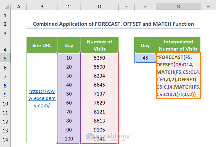
Method 5 – Combined Application of FORECAST, OFFSET, and MATCH Functions
- Use the following formula for the result cell:
=FORECAST(F5,OFFSET(D5:D14,MATCH(F5,C5:C14,1)-1,0,2),OFFSET(C5:C14,MATCH(F5,C5:C14,1)-1,0,2))
In the above formula, OFFSET(D5:D14,MATCH(F5,C5:C14,1)-1,0,2) syntax specifies the reference for the dependent values (known_y’s). Here, the MATCH function finds the relative position of the lookup value (F5 cell) for which you want to interpolate. Besides, 0 is the Cols (column) argument of the OFFSET function. It is zero as you are going to interpolate in the same column. Besides, the value of the Height argument is 2 because you want to interpolate for the last 2 values.
The OFFSET(C5:C14,MATCH(F5,C5:C14,1)-1,0,2)) formula returns the reference for the independent variables (known_x’s).
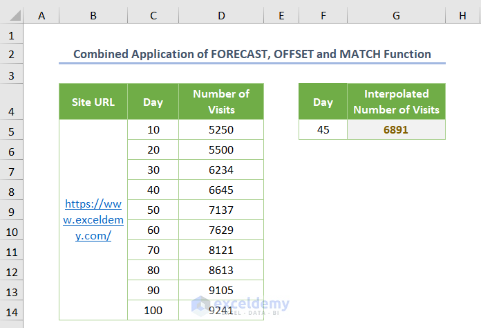
The FORECAST function interpolates the Number of Visits for Day 45 (listed in cell F5).
You’ll get the following output.
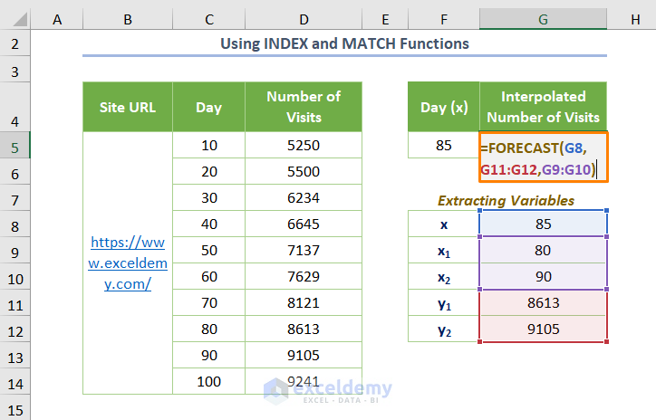
Method 6 – Using INDEX and MATCH Functions to Do Linear Interpolation
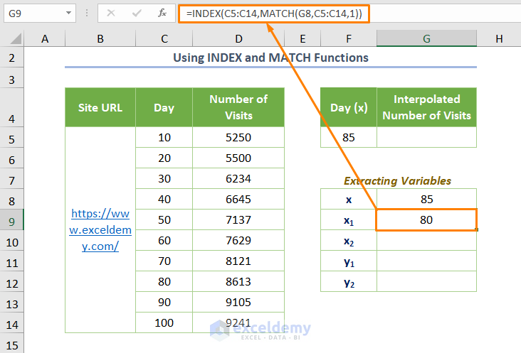
- Use the following formula for x1:
=INDEX(C5:C14,MATCH(G8,C5:C14,1))
Here, G8 is the value of Day 85 (x) for which you want to interpolate. The above formula finds the value of x1 where the MATCH function returns the relative position of the lookup value. 1 is used to find the lower value if the exact value is not found. Finally, the INDEX function returns the matched value from the known_y’s.
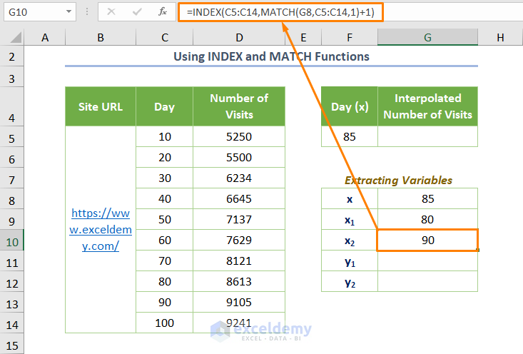
- Use the following formula for x2:
=INDEX(C5:C14,MATCH(G8,C5:C14,1)+1)
Here, 1 is added to find the higher value than the lookup value especially if exact matching is not found.
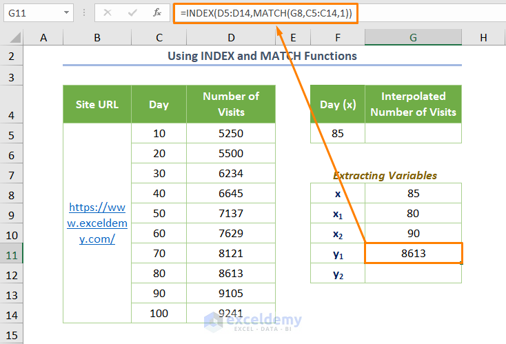
- Use the following formula for y1:
=INDEX(D5:D14,MATCH(G8,C5:C14,1))
The same thing happens here except for dealing with the independent range of data.
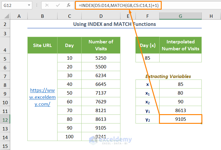
- Use the following formula for y2:
=INDEX(D5:D14,MATCH(G8,C5:C14,1)+1)
- Finally, copy the following function to interpolate based on the found values of x1,x2, and y1,y2:
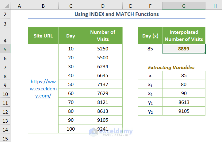
=FORECAST(G8,G11:G12,G9:G10)
Here, G11:G12 is the cell range of known_y’s and G9:G10 is for the known_x’s.
You’ll get the following output.
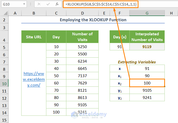
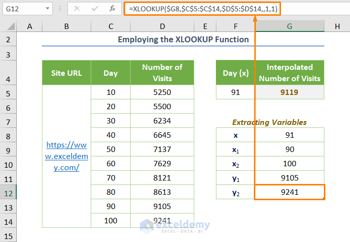
Method 7 – Using the XLOOKUP Function to Do Linear Interpolation in Excel
Available from Excel for Microsoft 365 and Excel 2021.
- Use the following formula for x1:
=XLOOKUP($G8,$C$5:$C$14,C$5:C$14,,-1,1)
Here, -1 (the value of the match_mode argument) is for finding the next smaller item and 1 is for searching from the top of the array (search_mode argument)

- Use the following formula for x2:
=XLOOKUP($G8,$C$5:$C$14,C$5:C$14,,1,1)
Here, 1 (the value of the match_mode argument) is for finding the next largest value.
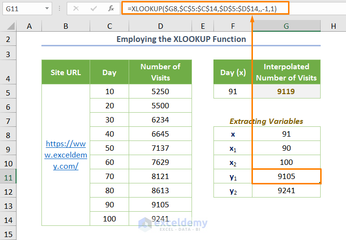
- Use the following formula for y1:
=XLOOKUP($G8,$C$5:$C$14,$D$5:$D$14,,-1,1)
This formula is the same as the earlier one. The only exception is here i.e. dealing with the dependent range of data.
- Use the following formula for y2:
=XLOOKUP($G8,$C$5:$C$14,$D$5:$D$14,,1,1)
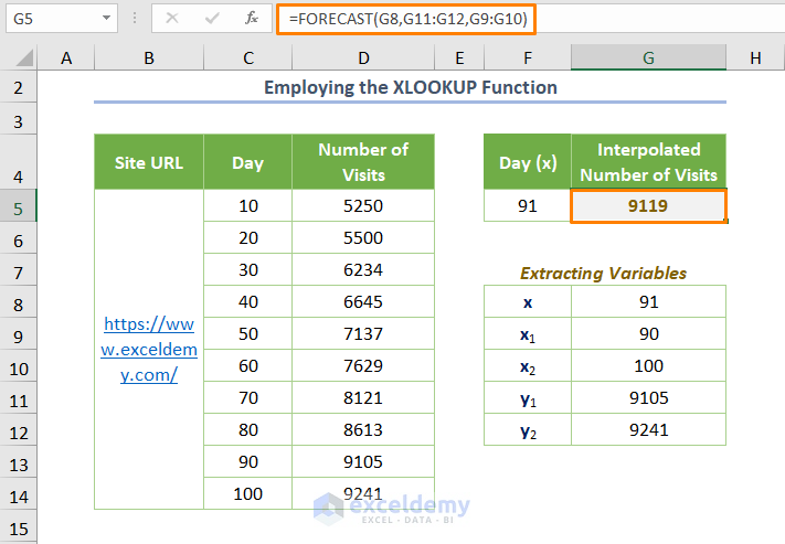
- Use the FORECAST function to interpolate and you’ll get your desired output:
=FORECAST(G8,G11:G12,G9:G10)
Read More: How to Do VLOOKUP and Interpolate in Excel
Things to Remember
- If the value of the x is non-numeric, you’ll get #VALUE! Error in the case of using the FORECAST function.
- If the cells of known_x’s and known_y’s are empty, you’ll get a #N/A error.
Download Practice Workbook
Related Articles
- How to Interpolate Missing Data in Excel
- How to Interpolate Between Two Values in Excel
- How to Perform Bilinear Interpolation in Excel
- How to Use Non Linear Interpolation in Excel
- How to Interpolate in Excel Graph
- How to Do Interpolation with GROWTH & TREND Functions in Excel
- How to Do Linear Interpolation Excel VBA
<< Go Back to Excel Interpolation | Excel for Statistics | Learn Excel
Get FREE Advanced Excel Exercises with Solutions!
