How to Perform Bilinear Interpolation in Excel (Easy Steps)

Bilinear interpolation is a technique used to estimate function values for two variables when the actual function is unknown. In Microsoft Excel, you can perform bilinear interpolation more easily than in Matlab.

What Is Bilinear Interpolation?

When you want to find the value of a function f(x,y) having two variables, bilinear interpolation is a method of estimating the value even when the proper function is unknown. Suppose you have only two variables and their output, but you do not know the equation of the function. Bilinear interpolation helps you estimate the output of two input variables.

The equation for bilinear interpolation is given below:

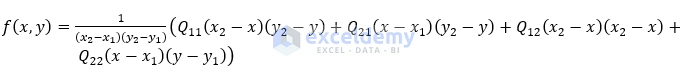
Here,

x = input value of x

y = input variable y

x_1 = very close adjacent below value of x from given data

x_2 = very close adjacent above value of x from given data

y_1 = very close adjacent below value of y from given data

y_2 = very close adjacent above value of y from given data

q_11 = function value of x_1, y_1

q_12 = function value of x_1, y_2

q_21 = function value of x_2, y_1

q_22 = function value of x_2, y_2

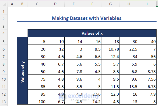
Step 1 – Creating a Dataset with Variables

Create a dataset with function values for different variable pairs. Ensure the input data is in increasing order.

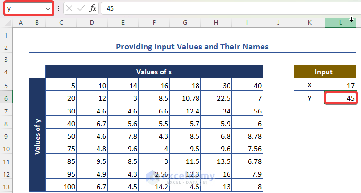
Step 2 – Providing Input Values and Their Names

• Given an input value of 17, name it x.

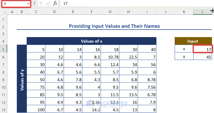
• Provide an input value for y (you’ve taken x), and name it accordingly.

Read More: How to Do Linear Interpolation in Excel

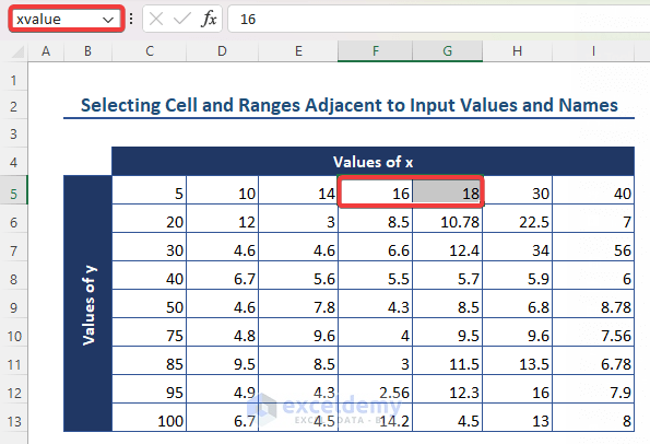
Step 3 – Selecting Cells Adjacent to Input Values and Names

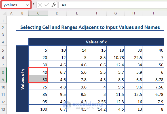
• For input x = 17 and y = 45, select adjacent values: x = 16 to x = 18 and y = 40 to y = 50.
• Name these ranges as xvalue and yvalues.

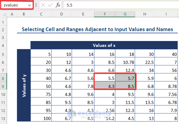
• Now, select the corresponding function values and name them zvalues.

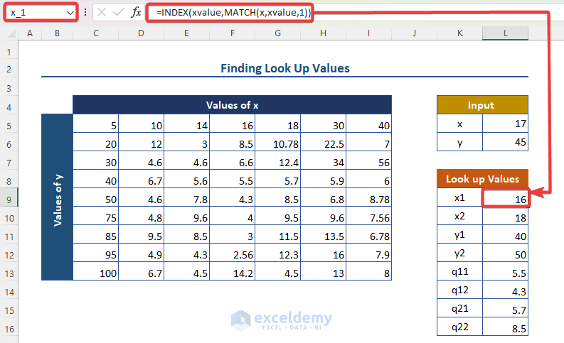
Step 4 – Finding Look Up Values

• Use INDEX and MATCH functions to find:
  • x_1 (just below desired x-value of 235): =INDEX(xvalue, MATCH(x, xvalue, 1)).

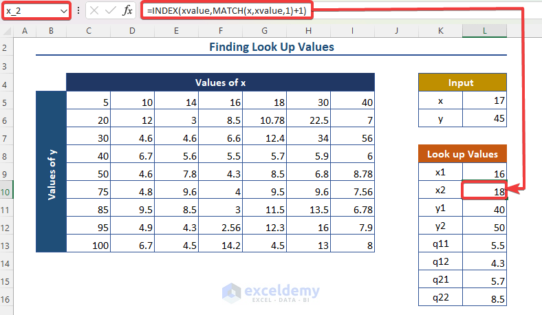
• • x_2 (just above desired x-value): =INDEX(xvalue, MATCH(x, xvalue, 1) + 1).

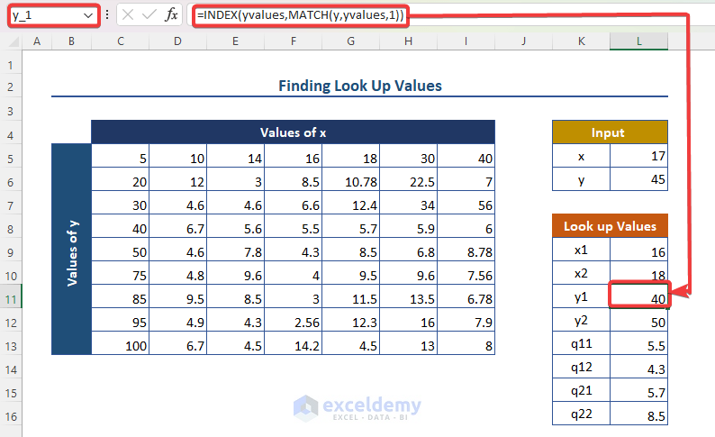
• • y_1 (similar process as x_1): =INDEX(yvalues, MATCH(y, yvalues, 1)).

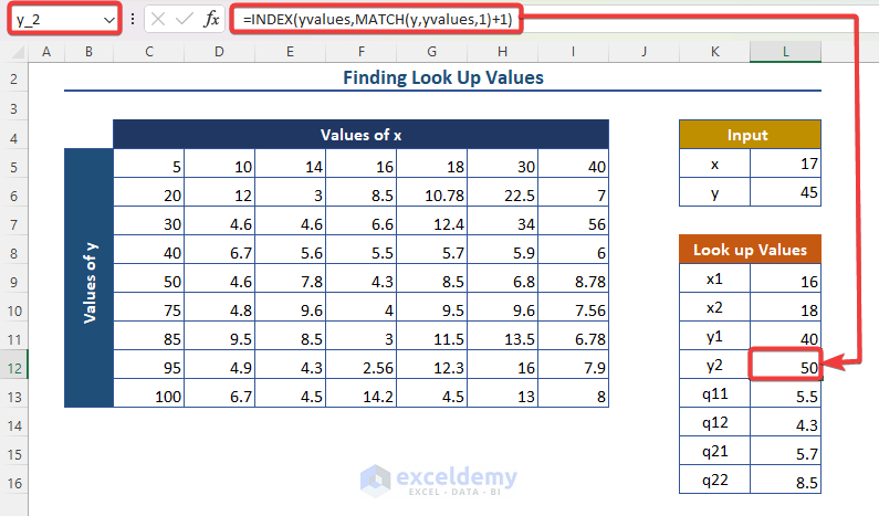
• • y_2 (similar process as x_2): =INDEX(yvalues, MATCH(y, yvalues, 1) + 1).

• • q_11 (function value at x_1, y_1): =INDEX(zvalues, MATCH(y_1, yvalues, 0), MATCH(x_1, xvalue, 0)).

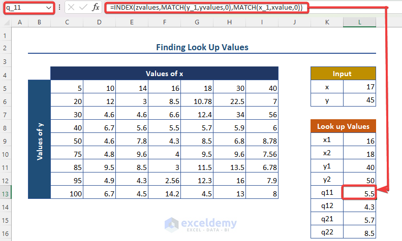
• • q_12 (similar process as q_11): =INDEX(zvalues, MATCH(y_2, yvalues, 0), MATCH(x_1, xvalue, 0)).

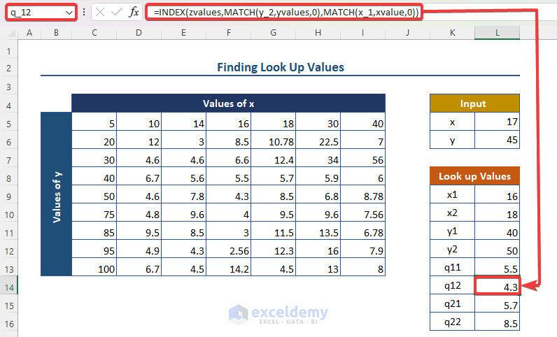
• • q_21 (similar process as q_11): =INDEX(zvalues, MATCH(y_1, yvalues, 0), MATCH(x_2, xvalue, 0)).

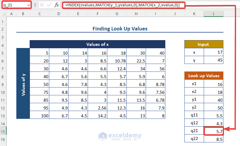
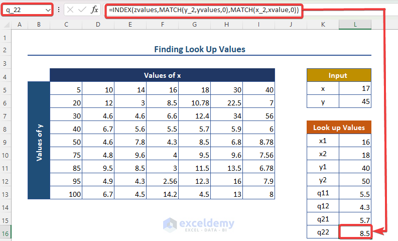
• • q_22 (similar process as q_11): =INDEX(zvalues, MATCH(y_2, yvalues, 0), MATCH(x_2, xvalue, 0)).

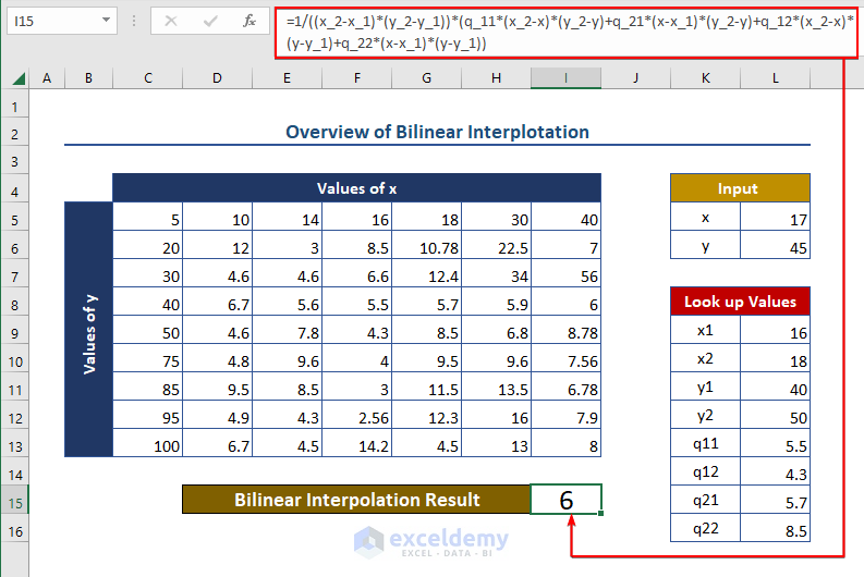
Step 5 – Showing Final Results

We calculate the final result using the lookup values and input x and y. The bilinear interpolation formula is as follows:

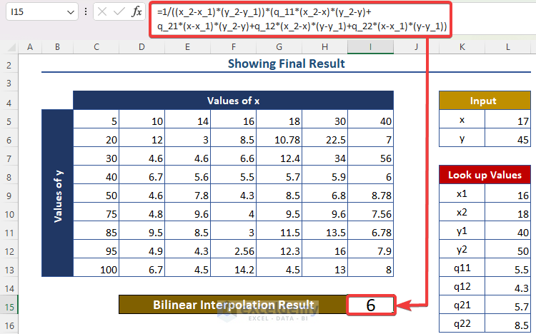
Read More: How to Use Non-Linear Interpolation in Excel

Download Practice Workbook

You can download the practice workbook from here:

Related Articles

• How to Interpolate Missing Data in Excel
• How to Do VLOOKUP and Interpolate in Excel
• How to Do Interpolation with GROWTH & TREND Functions in Excel
• How to Interpolate Between Two Values in Excel
• How to Interpolate in Excel Graph
• How to Do Linear Interpolation Excel VBA

<< Go Back to Excel Interpolation | Excel for Statistics | Learn Excel