How to Do 2D Interpolation in Excel (2 Suitable Ways)

In this article, we will show how to do 2D interpolation in Excel. It is possible to do the task of interpolation for both linear and non-linear datasets. You can easily interpolate in Excel if you properly follow the steps. The steps are quite simple. So, without any delay, let’s start the discussion.

2D Interpolation in Excel: 2 Suitable Ways

We can easily do 2D interpolation in Excel. There can be 2 types of interpolation. We can interpolate for linear data and also for non-linear data. Here, we will show you how to do 2D interpolation for both linear and non-linear methods.

1. Perform Interpolation of Linear 2D Data in Excel

It is easy to perform interpolation of linear 2D data in Excel. We will show you 5 ways. Each method is quite easy. You can follow any process to do the task. To demonstrate the methods we will use the following dataset. In the dataset, there is information on the weekly sales of a shop. Here, sales records are for odd weeks. By interpolation, you can find sales of any even weeks. We will find an in-between sales value for week 8. Let’s follow the steps below to learn these methods.

1.1 Apply Mathematical Equation for Linear Interpolation

There is an established mathematical equation for linear equations.

y= y1 + (x-x1)⨯(y2-y1)/(x2-x1)

Using this mathematical equation, we can easily interpolate linear data. So, follow the steps below to learn the method.

STEPS:

Firstly, find out the coefficients of this equation.
So, place the values of x1, x2, y1, y2, and x in the Excel Sheet.

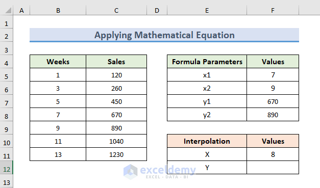
Here, we want to find out the sales for the week of 8. So, x = 8. In the dataset, there is sales information for 7 and 9. So, x1 = 7 and x2 = 9. And y represents the corresponding sales of these weeks. For this reason, y1 = 670 and y2 = 890.

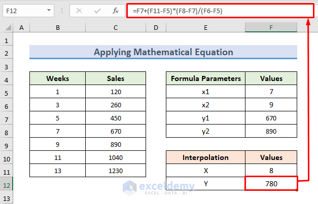
Then, write down the following formula in the F12 cell:

=F7+(F11-F5)*(F8-F7)/(F6-F5)

Then, press Enter to observe the interpolated result.

1.2 Interpolate Using Trendline in Excel

The trendline is one of the easiest methods for interpolating a linear equation. From the trendline, we can plot a linear line. And from this line, we can interpolate data.

STEPS:

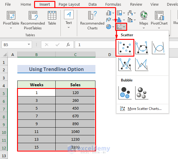
Firstly, we have to insert a plot from the dataset.
To do so, click on the Insert tab.
After that, click on the drop-down menu of the Insert Scatter (X, Y) or Bubble Chart from the Charts group.
Instantly, a wizard will come out.
From the wizard, select the Scatter chart.

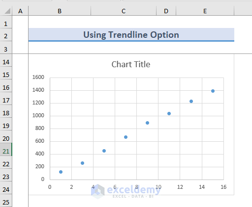
As a result, the following chart is shown on the Excel Sheet.

In the following step, we will insert Trendline.
To do so, click on the chart.
Therefore, you can see a plus (+) icon.
So, click on this icon and give a tick on the Trendline.

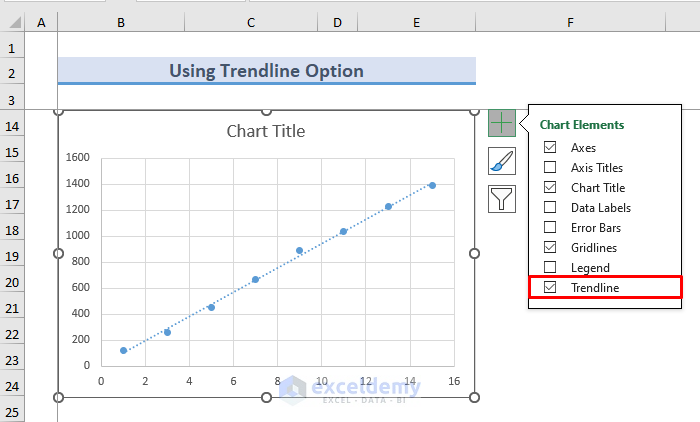
As a result, a trendline can be seen on the chart.
Now, double-click on the trendline.
Instantly, the Format Trendline window will appear on the right side of the Excel Sheet.
Then, give a tick on Display Equation on chart.
After that, look at the chart and you can see a floating equation.

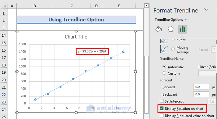
So, you can find the value of y from this equation.
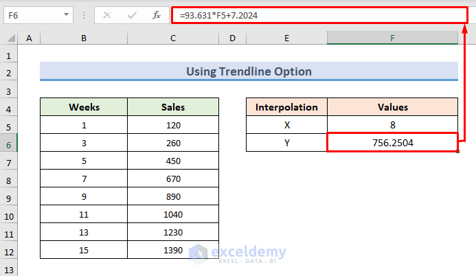
Now, according to the equation, write down the following formula in the F6 cell:

=93.631*F5+7.2024

Then, press Enter to observe the interpolated result of sales.

1.3 Interpolate 2D Data Using SLOPE and INTERCEPT Functions

We can also build up a formula using the Slope function and the Intercept function.

There is an established mathematical equation for linear equations.

y= mx+c

Using this equation, we will interpolate the 2D data.

STEPS:

Here, we need to find out the co-efficient of m and c for interpolation.
Now, write down the following formula in the F6 cell:

=SLOPE(C5:C12,B5:B12)*F5+INTERCEPT(C5:C12,B5:B12)

Then, press Enter to observe the interpolated result.

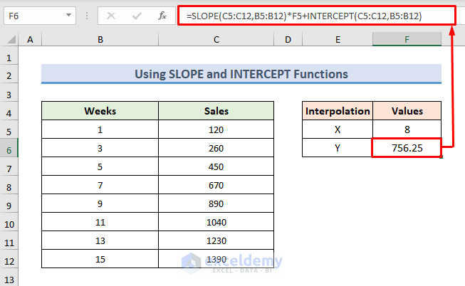
Here, we want to find out the sales for the week of 8. So, x = 8. “M” denotes the slope of the straight line. And, c represents the interception of the straight line with the vertical axis. With the SLOPE function, we have calculated the slope. And, the INTERCEPT function calculates the interception.

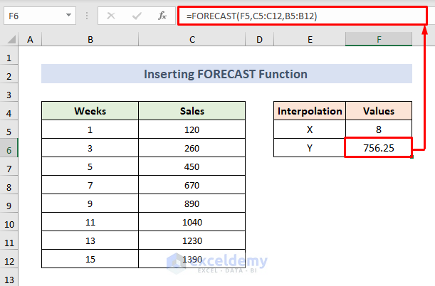
1.4 Insert FORECAST Function for Interpolation

Interpolation is one kind of forecasting as we are predicting or anticipating the value. We don’t exactly know the real value exists. So, Excel’s in-built the FORECAST Function comes in quite handy in this regard.

STEPS:

Now, write down the following formula in the F6 cell:

=FORECAST(F5,C5:C12,B5:B12)

Then, press Enter to observe the interpolated result.

1.5 Interpolation of 2D Data Using TREND Function

Using the TREND Function, it is quite simple to interpolate from the linear data.

STEPS:

Now, write down the following formula in the F6 cell:

=TREND(C5:C12,B5:B12,F5,1)

Then, press Enter to observe the interpolated result.

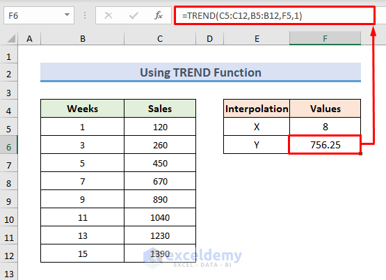
Here, in the TREND function, we have set the constant 1. Here, the TREND function predicts the linear trend of the dataset.

2. Do Interpolation of Non-Linear 2D Data in Excel

It is easy to perform interpolation of non-linear 2D data in Excel. We will show you 2 ways. Each method is quite easy. You just need to insert the formula. Here, you can follow any method to do the task. To demonstrate the methods we will use the following dataset. In the dataset, there is information on the weekly sales of a shop. Here, sales records are for odd weeks. By interpolation, you can find sales of any even weeks. We will find an in-between sales value for week 8. Let’s follow the steps below to learn these methods.

2.1 Interpolation in 2D Using GROWTH Function

Excel has another built-in function called GROWTH. The GROWTH function is more reliable and accurate for exponential and non-linear datasets.

STEPS:

Now, write down the following formula in the F6 cell:

=GROWTH(C5:C12,B5:B12,F5,2)

Then, press Enter to observe the interpolated result.

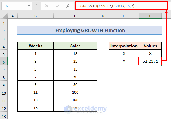
Here, in the GROWTH function, we have set the constant 2.

2.2 Combine FORECAST, INDEX, and MATCH Functions for Non-Linear Interpolation

Finding non-linear data is very difficult compared to linear data because it is difficult to find the pattern. The FORECAST function shows good results for interpolating linear datasets. But for the non-linear datasets, the result is not up to the mark. And the GROWTH function works well for the exponential dataset. For this reason, we have formulated a new formula combining the FORECAST, INDEX and MATCH functions.

STEPS:

Now, write down the following formula in the F6 cell:

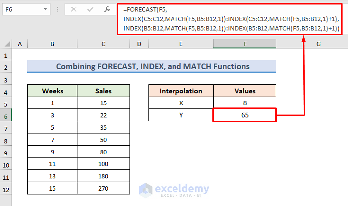
=SLOPE(C5:C12,B5:B12)*F5+INTERCEPT(C5:C12,B5:B12)

Then, press Enter to observe the interpolated result.

Here, we use the MATCH function to retrieve the positions of the value close to 8. Then, we have used the INDEX function to determine the cell reference for that value. Then, we have created a dynamic range and the FORECAST function predicts the interpolated value from this dynamic range.

Download Practice Workbook

To practice by yourself, download the following workbook.

2D Interpolation.xlsx

Conclusion

In this article, we have demonstrated how to do 2D interpolation in Excel. There is a practice workbook at the beginning of the article. Go ahead and give it a try. Last but not least, please use the comment section below to post any questions or make any suggestions you might have.

<< Go Back to Excel Interpolation | Excel for Statistics | Learn Excel

Get FREE Advanced Excel Exercises with Solutions!

How to Do 2D Interpolation in Excel (2 Suitable Ways)

2D Interpolation in Excel: 2 Suitable Ways

1. Perform Interpolation of Linear 2D Data in Excel

1.1 Apply Mathematical Equation for Linear Interpolation

1.2 Interpolate Using Trendline in Excel

1.3 Interpolate 2D Data Using SLOPE and INTERCEPT Functions

1.4 Insert FORECAST Function for Interpolation

1.5 Interpolation of 2D Data Using TREND Function

2. Do Interpolation of Non-Linear 2D Data in Excel

2.1 Interpolation in 2D Using GROWTH Function

2.2 Combine FORECAST, INDEX, and MATCH Functions for Non-Linear Interpolation

Conclusion

Related Articles

Leave a reply Cancel reply