Microsoft Excel allows us to estimate different types of data and carry out monetary, mathematical, and statistical computations. Excel is a great tool for interpolation as it essentially performs as a large visual calculator. Interpolation is the method of calculating unknown points within an existing known data set. When we try to find unknown values of a function between two known values, interpolation is used. Excel allows us to perform interpolation, both linear and exponential, in an easier way. In this article, I will try to explain a couple of ways to calculate exponential interpolation in Excel.
Performing Exponential Interpolation in Excel: 4 Easy Ways
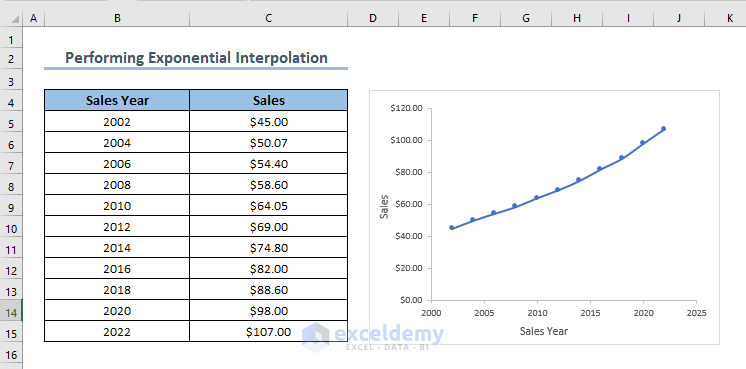
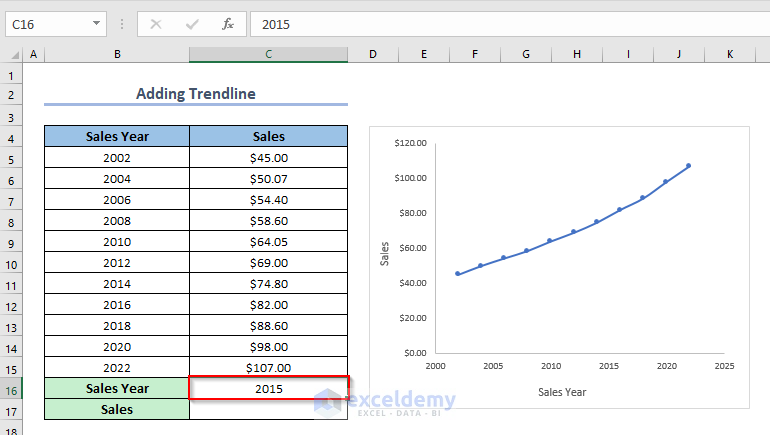
In the case of a real-world dataset where the values are exponential, we can use different Excel Functions to perform the interpolation. In this article we are going to use Excel 365 version, you can use any other version as well. Here, we will discuss 4 effective ways of exponential interpolation. We will use the following exponential dataset to show the ways of interpolation in Excel.
In this dataset, there are a total of 2 columns of Sales Year & Sales and 12 rows. Here the Sales Year column denotes X coordinate values and the Sales column denotes Y coordinate values. As we can see these values are generating an exponential graph for which we will perform our interpolation.
1. Using GROWTH Function to Perform Exponential Interpolation
The GROWTH function in Excel allows us to interpolate data when the data set has exponential growth. It uses exponential regression to predict a value. In our dataset, the values of the X coordinate and Y coordinate have a linear relation between them.
Steps:
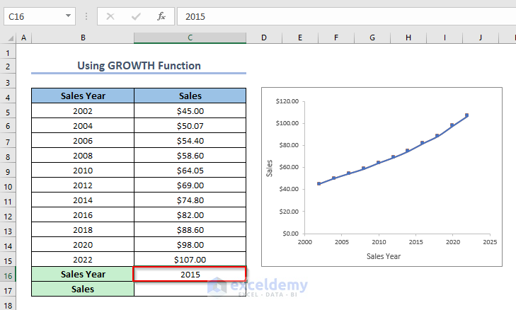
- Select cell C16 and enter the sales year of which we want to know the sales value. Let it be 2015.
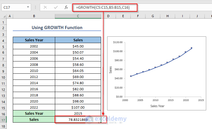
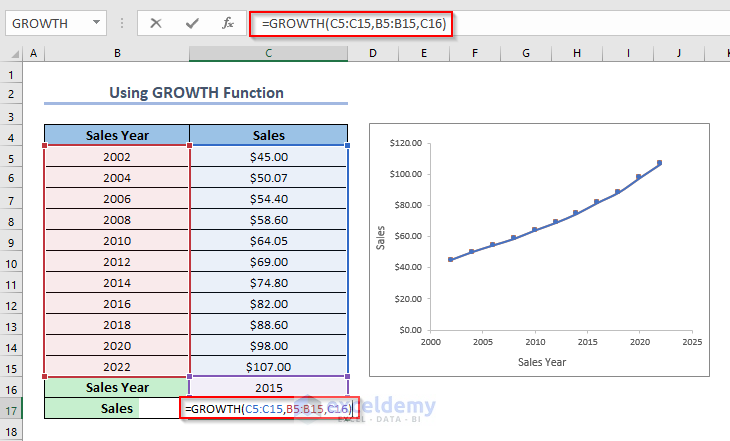
- Select cell C17 and then type the following formula.
=GROWTH(C5:C15,B5:B15,C16)Here, in the first argument enter the range of cells of known y-values, in the second argument, the range of cells of known x-values, and in the last argument enter the new x-value for which you want to know the y-value. In this dataset, X coordinate values denote the Sales Year column, and Y coordinate values denote the Sales column.
- Press ENTER key and the result will be shown in cell C17.
Here, we got the Sales value for the year 2015.
2. Adding Trendline for Exponential Interpolation in Excel
In Excel, we can utilize the Trendline feature when the dataset is non-linear. The Exponential Trendline is an angled line that illustrates an increasing increase or decrease in data values. However, we have to keep in mind that we cannot create an Exponential Trendline for the dataset that has negative values or zeros.
Steps:
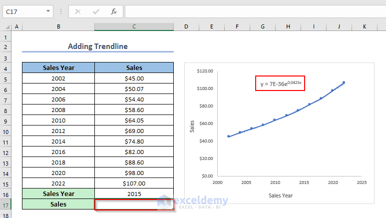
- Select cell C16 and enter the sales year for which we want to know the sales value using the Trendline feature. Let it be 2015.
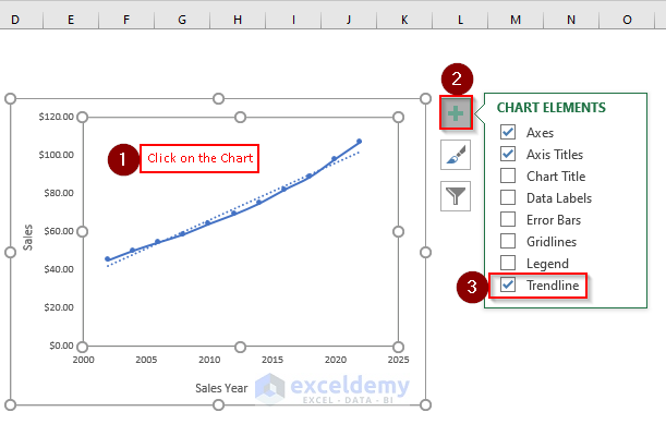
- Click on the chart and then click on the plus symbol which is CHART ELEMENTS.
- Click on the check mark beside Trendline, and we will get the dotted curve line in our chart.
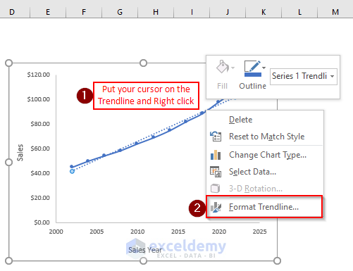
- After that put your cursor on the Trendline and right-click on your mouse.
- Click Format Trendline.
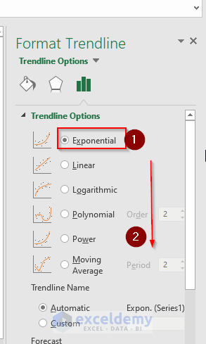
- After clicking Format Trendline, you will get the Format Trendline dialog box.
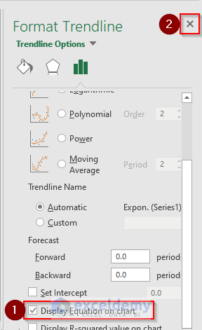
- Select Exponential and scroll down.
- Click on the check mark beside Display Equation on chart.
- Click Close.
- We will get our desired equation that we can use in C17.
The equation is like this below.
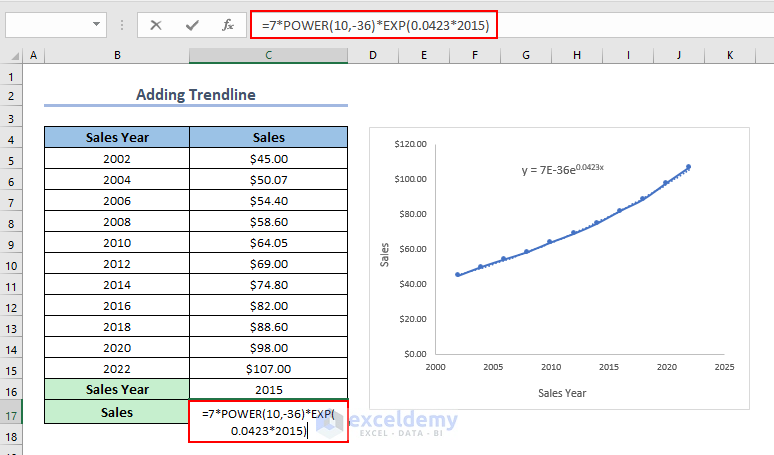
- Select cell C17 and then type the following equation.
=7*POWER(10,-36)*EXP(0.0423*2015)Formula Breakdown
- POWER(10,-36) → The POWER function will return the result of the number 10 raised to the power -36. Here, 10 is the number, and -36 is the power value.
- Output → 1E-36
- 7*POWER(10,-36) → becomes
- 7*1E-36
- Output → 7E-36
- 7*1E-36
- EXP(0.0423*2015) → The EXP function will return e raised to the power of number 2015.
- Output → 03961615076379E+37
- 7*POWER(10,-36)*EXP(0.0423*2015) → becomes
- 7*7E-36*1.03961615076379E+37
- Output → 72.77313055
- 7*7E-36*1.03961615076379E+37
- Press ENTER key, and the result will be shown in cell C17.

Here, we got the Sales value of 2015.
3. Applying FORECAST Function for Exponential Interpolation in Excel
The FORECAST function in Excel is widely used to predict performance by analyzing a set of real-world data points. This is used to determine or estimate a future value based on previous values; the predicted value is a y-value for a given x-value.
It is to notify you that to make room for the new Forecasting functions, the FORECAST function in Excel 2016 was replaced with the FORECAST.LINEAR function. If you are going to use a version of Excel older than 2016, you can only use the FORECAST function since Microsoft Excel added FORECAST.LINEAR in the 2016 version.
Steps:
- Select cell C16 and ENTER the sales year of which we want to know the sales value using the FORECAST function. Let it be 2015.

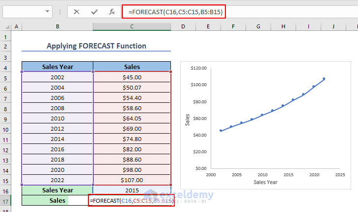
- Select cell C17 and then type the following formula.
=FORECAST(C16,C5:C15,B5:B15)Here, in the first argument enter the x-value for which you want to know the y-value, in the second argument enter the range of cells of known y-values, and in the last argument, the range of cells of known x-values. In this dataset, X coordinate values denote the Sales Year column and Y coordinate values denote the Sales column.
- Press ENTER key, and the result of Sales will be shown in cell C17.
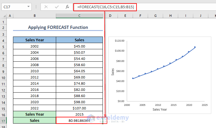
Here, in cell C17 we got the sales value of 2015.
The FORECAST and FORECAST.LINEAR functions are effectively the same. So, you can utilize that as well. The result will be the same as before.
For that, the following formula will be generated in cell C17 as
=FORECAST.LINEAR(C16,C5:C15, B5:B15)
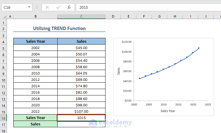
4. Utilizing TREND Function for Exponential Interpolation in Excel
The TREND Function is an Excel Statistical function that estimates an unknown value based on linear regression. Here, for this dataset, you can use the TREND function of Excel.
Steps:
- Select cell C16 and enter the sales year of which you want to know the sales value using the TREND function. Let it be 2015.
- Select cell C17 and then type the following formula.
=TREND(C5:C15,B5:B15,C16)Here, in the first argument enter the range of cells of known y-values, in the second argument, the range of cells of known x-values, and in the last argument enters the x-value for which you want to know the y-value. As you already know that in the dataset X coordinate values denote the Sales Year column and Y coordinate values denote the Sales column.
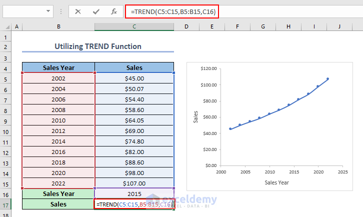
- Press ENTER Key, and the result will be shown in cell C17.

Here, in cell C17 we got the sales value of 2015.
Practice Section
You can use the following dataset to practice by yourself. Hope it will help you to learn more.

Download Practice Workbook
Conclusion
This article will help you to understand how to use different functions to perform exponential interpolation in Excel. You can use these 4 effective ways to calculate interpolation when you have a real-world dataset. I hope you have found this article interesting as well as effective. If you face any difficulties understanding any topic, please leave a comment in the comment section below and give us your feedback.
Related Articles
- How to Do 2D Interpolation in Excel
- 3D Interpolation in Excel
- How to Do Polynomial Interpolation in Excel
- How to Calculate Logarithmic Interpolation in Excel
- How to Interpolate Time Series in Excel
- How to Apply Cubic Spline Interpolation in Excel
<< Go Back to Excel Interpolation | Excel for Statistics | Learn Excel
Get FREE Advanced Excel Exercises with Solutions!
