To understand an Excel chart well, I will advise you to know the Excel chart elements very well. It is very important to be introduced to the parts of charts in Excel. This article will give you the full guide. Let’s start…
Create a Chart in Excel
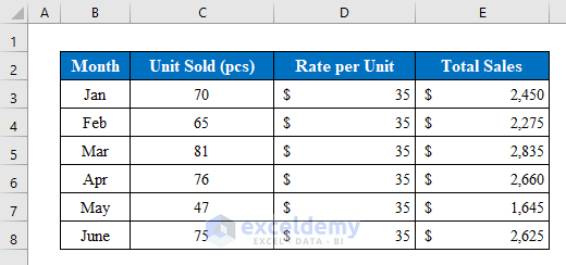
To introduce you to the different parts of an Excel chart, I have used the following data table. Suppose we have a dataset of some Products Month-wise Sales, Unit Price per Piece, and Total Sales. Now we will create a chart and then utilize all the chart elements.
Steps:
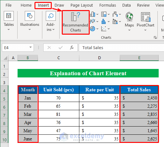
- Starting with, choose data from the dataset and press “Recommended Charts” from the “Insert” option.
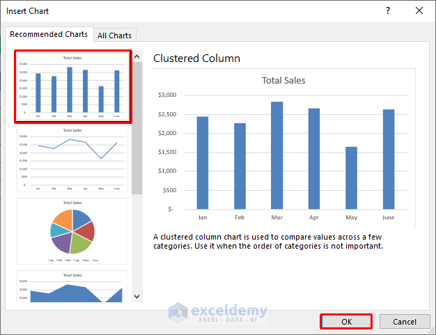
- From the new window select any chart of your choice and press OK to continue.
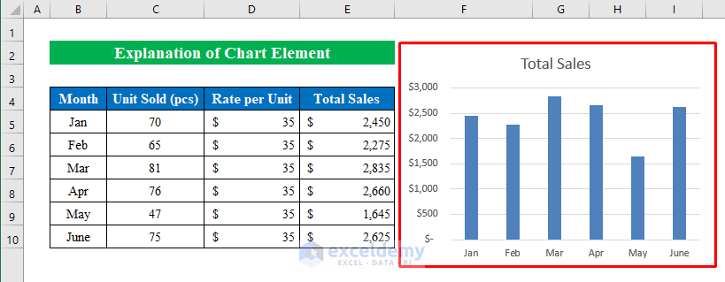
- Finally, you will get a chart inside the worksheet.
How to Use Chart Elements in Excel: 9 Different Examples
Now we will learn about all the chart elements in this part. With the help of the chart element, you can give a new descriptive look to your chart which will make your chart more appealing. Stay tuned!
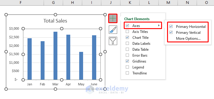
1. Use Axes in Chart Elements
This chart has a horizontal axis. The horizontal axis is known as the category axis. This axis holds the Month column information.
It has two vertical axes. Vertical axes are known as value axes. Each axis has a different scale. The left axis holds the Sales data series. The value axes also display scale values. The left vertical axis shows scale values from 0 to $3,500, incremented by 500.
2. Apply Different Axis Titles
If you want you can change the axis title from the chart element in Excel.
Steps:
- Just click the plus sign (+) that appeared on the right side of the chart and then click “Axis Titles“.
- Now from the drop-down list, you will get “Primary Horizontal” and “Primary Vertical” as we have two axis in this chart.
- Hence, choose any name in the axis title according to your choice.
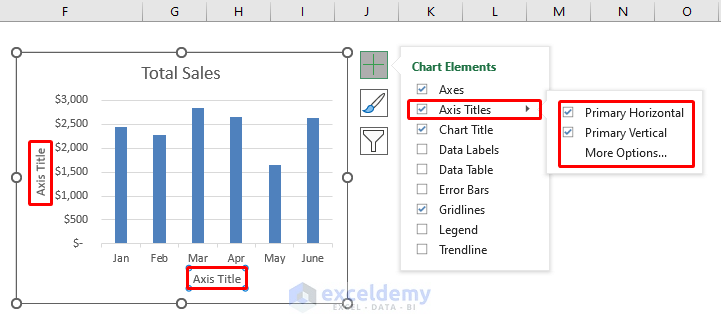
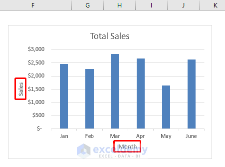
- Here, I have named the “Primary Horizontal” axis as “Month” and the “Primary Vertical” as “Sales“.
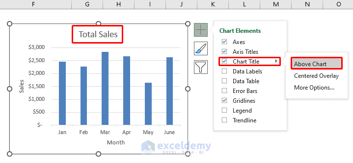
3. Use Chart Titles Option
Here in this chart, the chart title is “Total Sales“. You can change or remove it utilizing the “Chart Title” option.
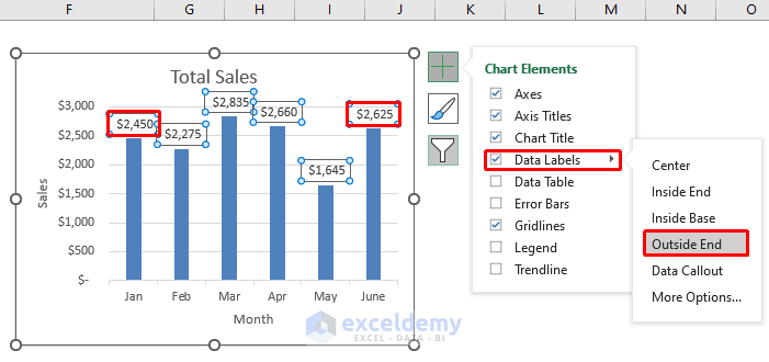
4. Appy Data Labels with Multiple Criteria
While working with a chart you might feel the need to add data labels inside the chart. In that situation, use the “Data Labels” option from the chart element icon and add the data labels anywhere you want. You can add at “Center“, Inside End“, “Outside End“, and “Data Callout” positions. In the below screenshot I have added data labels to the “Outside End” of every data bar.
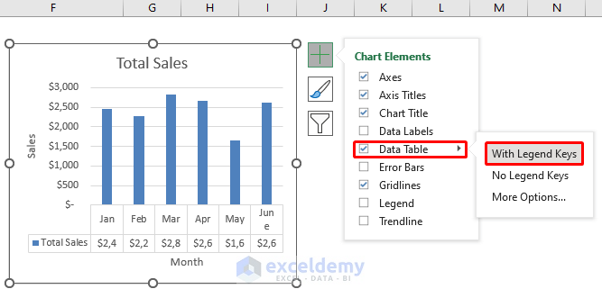
5. Insert Data Table from Chart Elements
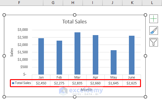
You can add a data table from the chart element option in Excel. Select the chart and from the drop-down list choose your desired data table with “Legend keys” and “No Legend Keys“.
After checking and marking the option, the final chart will look like the following.
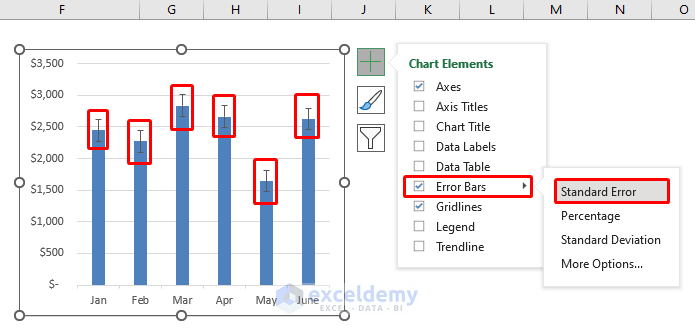
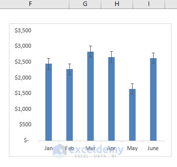
6. Apply Error Bars from Chart Elements
Sometimes your boss might want you to add error bars inside a chart so that the gap in sales can be seen inside the chart. Simply, checkmark the “Error Bars” option from the “Chart Elements” feature and visualize your data with a different look.
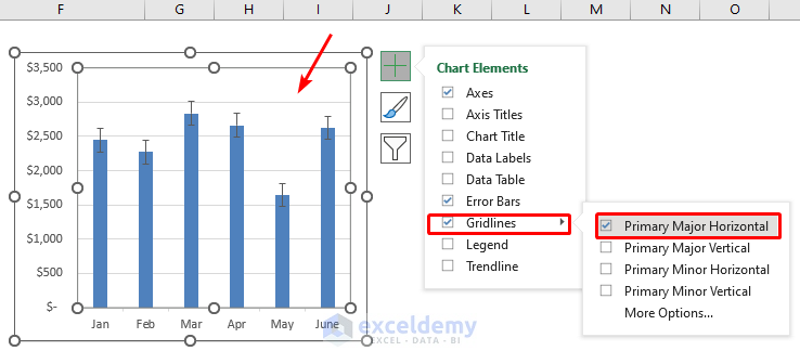
7. Use Gridlines Option in Excel
After creating a chart you might need to insert gridlines in your chart. Without gridlines, your chart will look exactly like the following.
Now from the chart elements option checkmark “Gridlines” and choose your precious gridlines from the list.
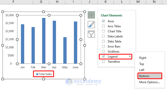
8. Insert Legend Option from Chart Elements
Legend can be named as the chart title in a chart. From the legend feature in chart elements, you can change the location of your main title at any position you want.
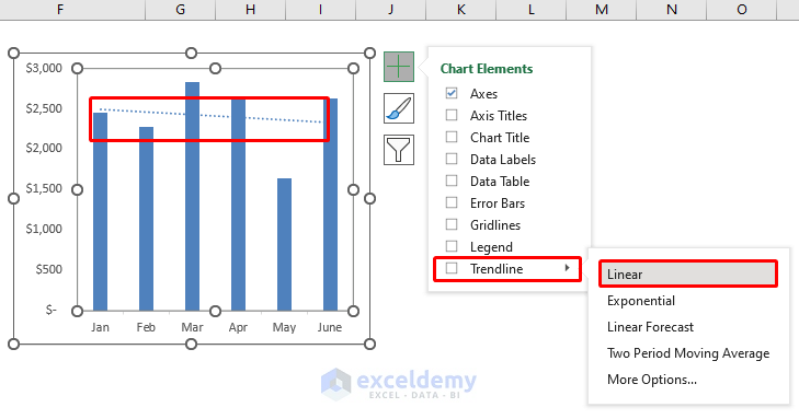
9. Apply Trendline Option to Show Tendency of Data in Excel
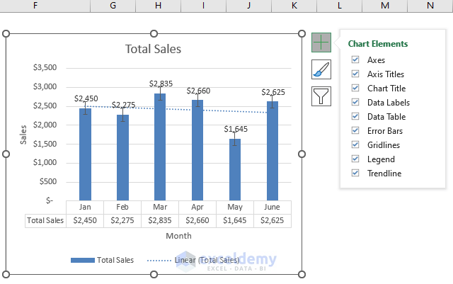
A trendline is a curved or straight line that displays the pattern or direction inside a chart. Utilizing the chart elements option you can add a trendline to your Excel chart. Just check mark the Trendline option and choose your desired trendline from the drop-down list. That’s it. Simple isn’t it?
After completing all the steps our final chart will look like the following screenshot.
Things to Remember
- If you don’t want to use any of the elements from the chart just remove the check mark from the list and it will automatically be removed from your chart.
Download Practice Workbook
Download this practice workbook to exercise while you are reading this article.
Conclusion
In this article, I have tried to cover all the ins and outs of chart elements in Excel. Take a tour of the practice workbook and download the file to practice by yourself. I hope you find it helpful. Please inform us in the comment section about your experience. We are always responsive to your queries. Stay tuned and keep learning.
Excel Chart Elements: Knowledge Hub
- Formatting Chart Elements in Excel
- Legend in Excel Chart
- Label Axis in Excel
- Format Axis in Excel
- Data Labels in Excel
<< Go Back To Excel Charts | Learn Excel
Get FREE Advanced Excel Exercises with Solutions!
