Method 1 – Scale Using Multiplication Symbol
Steps:
- Add a new cell named Scaling Factor.
- Insert a number on cell E5 as the scaling factor.
- Look at the formula of cell C5.
=B5*$E$5
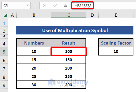
Use the multiplication symbol to scale based on the scaling factor. Use absolute reference as the scaling factor is fixed.
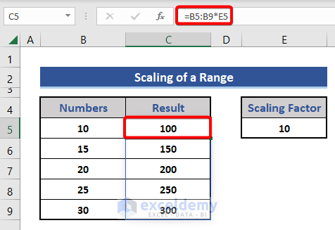
- Scale up a range with a single click. Look at the formula below.
=B5:B9*E5
Method 2 – Scaling Formula of One Range with Another Range
Steps:
- Look at the formula on cell D5.
- Use Range 2 column as the scaling factor for Range 1.
=B5:B9*C5:C9
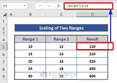
Do not need to apply the scaling factor for each cell of the Range 1 column separately.
Method 3 – Use of PRODUCT Function to Scale Data
Steps:
- Look at the following formula of cell C5.
=PRODUCT(B5,$E$5)
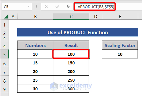
Use the absolute reference as the scaling factor is fixed.
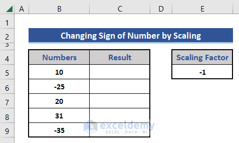
Method 4 – Change the Sign of the Number After Scaling
Steps:
- Modify the scaling factor and convert it to -1.
- Put the formula on cell C5.
=PRODUCT(B5,$E$5)
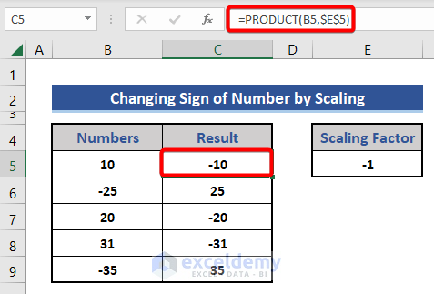
See the sign of numbers has been changed.
Use the following formula without using the cell reference of the scaling factor.
=PRODUCT(B5,-1)
Method 5 – Excel Scaling Formula to Scale Data from 0 to 1
Steps:
- Look at the formula of cell C5.
=(B5 - MIN(B:B)) / (MAX(B:B) - MIN(B:B))
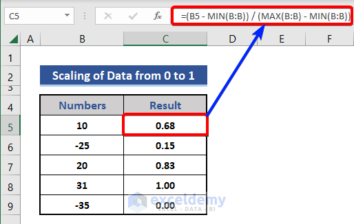
All the numbers are presented within the Range of 0 to 1. This is called normalized value.
Change the range, we have to multiply the formula using the biggest number of that range. If we want to scale numbers in the Range of 0 to 10, apply the following formula.
=10*(B5 - MIN(B:B)) / (MAX(B:B) - MIN(B:B))
Formula Explanation:
- MIN(B:B)
Get the minimum value of Column B.
Result: -35
- MAX(B:B)
Get the maximum value of Column B.
Result: 31
- B5 – MIN(B:B)
Subtract the minimum value of Column B from B5.
Result: 45
- MAX(B:B) – MIN(B:B)
Determine the difference between the minimum and maximum value of Column B.
Result: 66
- (B5 – MIN(B:B)) / (MAX(B:B) – MIN(B:B))
We perform a division operation in this section.
Result: 0.68
Method 6 – Calculating Standardized Values in Excel
Steps:
- Add two new rows for average value and deviation in the dataset.
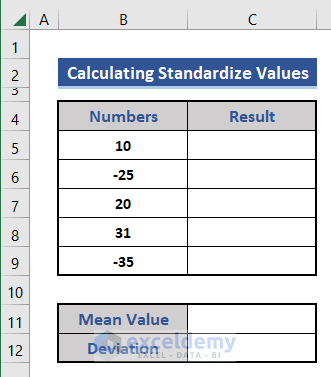
The average and deviation are the pre-requirement to calculate the standardized value in Excel.
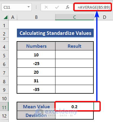
- We will use the AVERAGE function on the formula of cell C11 to calculate the mean value.
=AVERAGE(B5:B9)
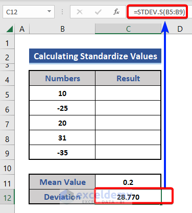
- Apply the STDEV.S function in cell C12 to calculate the standard deviation.
=STDEV.S(B5:B9)
- Put the following formula based on the STANDARDIZE function on cell C5.
=STANDARDIZE(B5,$C$11,$C$12)
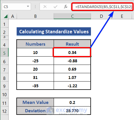
Get the standardized value after applying the formula. We used absolute reference as the average and mean values are fixed.
Download Practice Workbook
Download this practice workbook to exercise while you are reading this article.
Scaling Formula in Excel: Knowledge Hub
<< Go Back to Excel for Statistics | Learn Excel
Get FREE Advanced Excel Exercises with Solutions!
