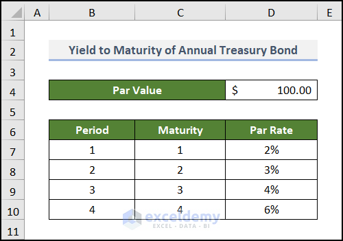
Example 1 – Bootstrapping Spot Rates for Annual Bond
The below dataset, Yield to Maturity of Annual Treasury Bond, includes the Par Value, Period, Maturity, and Par Rate in different columns.
1.1 Using Formula in Excel
Steps:
- Create a new column with the heading, Spot Rate under Column E.
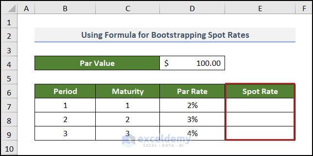
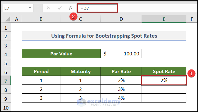
The Spot Rate for the 1st year should be the same as the Par Rate for this period.
- Select cell E7 and enter the cell reference of cell D7 with an equal sign.
=D7
- Press the ENTER key.
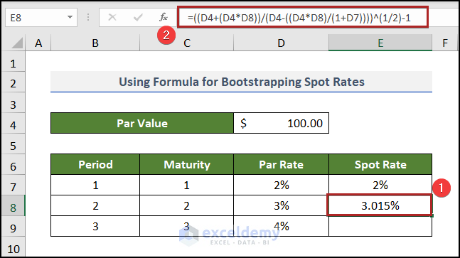
- Go to cell E8 and enter the following formula into the cell:
=((D4+(D4*D8))/(D4-((D4*D8)/(1+D7))))^(1/2)-1
- Press ENTER.
To get the Spot Rate for the 3rd year, solve the preceding equation. In Excel,
- Select cell E9 and insert the formula below:
=((D4+(D4*D9))/((D4-((D4*D9)/(1+D7))-((D4*D9)/(1+E8)^2))))^(1/3)-1
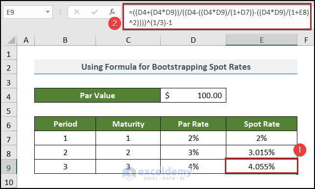
- Press ENTER.
1.2 Utilizing Solver Add-in
Steps:
The Spot Rate for year 1 in cell D11 is equal to the Par Rate of cell D7.
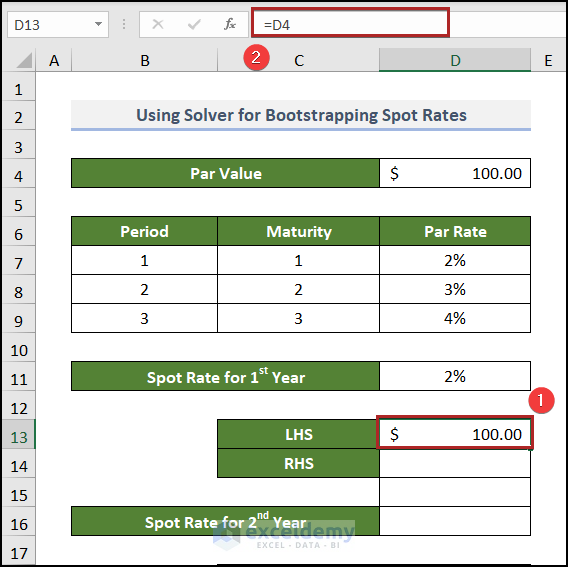
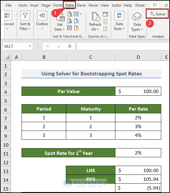
Now, we’ll form the equation in our Excel sheet. On the left-hand side, we placed 100.
- Go to cell D13 and enter the following cell reference:
=D4
- Press ENTER.
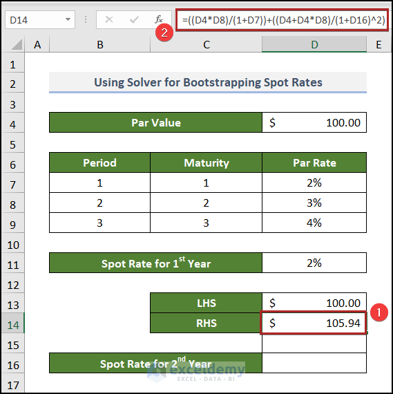
To insert the right-hand side of the equation,
- Go to cell D14 and write down the formula below:
=((D4*D8)/(1+D7))+((D4+D4*D8)/(1+D16)^2)
- Press ENTER.
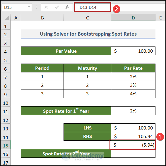
⇒ LHS = RHS
⇒ LHS – RHS = 0
Here, we applied this logic in cell D15.
=D13-D14
To get the value of the Spot Rate for 2nd Year in cell D16,
- Go to the Data tab.
- Click on Solver on the Analyze group of commands.
Note: If Solver isn’t available on your ribbon, you have to install the Solver add-in in Excel.
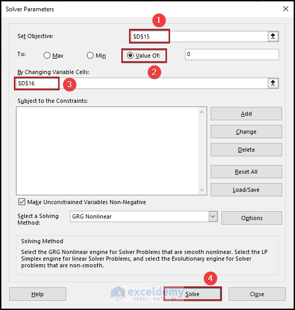
The Solver Parameters dialog box appears.
- In the Set Objective box, give the cell reference of cell D15.
- Select the Value of option.
- Place the cell reference of D16 in the By Changing Variable Cells box.
- Click on the Solve button.
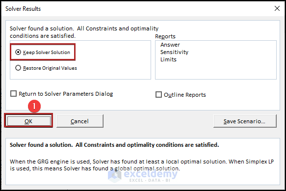
We can see the Solver Results wizard. The Keep Solver Solution option will be automatically selected.
- Click OK.
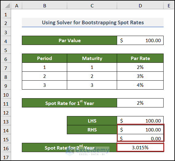
Here is the spot rate in cell D16. The values in cells in the D14:D15 range are automatically changed to make the two sides of the equation equal. The spot rate for the second year is 3.015%.
- See the formula to construct the equation for 3rd year in cell D19.
=((D4*D9)/(1+D7))+((D4*D9)/(1+D8)^2)+((D4+D4*D9)/(1+D21)^3)
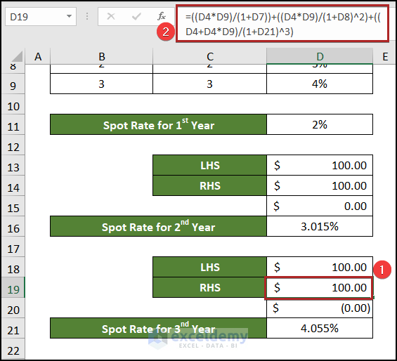
- Repeat the earlier steps to use the solver to solve the rate for this year.
Read More: How to Perform Bootstrapping in Excel
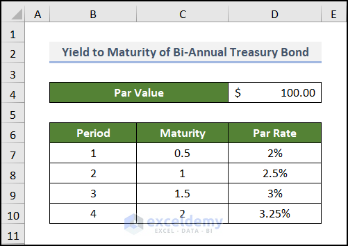
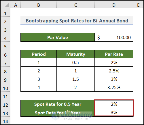
Example 2 – Bootstrapping Spot Rates for Bi-Annual Bond
In the below dataset we have a Yield to Maturity of Bi-Annual Treasury Bond. The maturity periods are 0.5 years, 1 year, 1.5 years, etc.
Steps:
The half-yearly and yearly Spot Rates would be the same as those periods’ Par Rates.
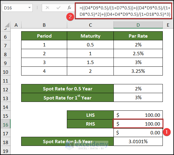
Here, we are giving the equation for the spot rate for 1.5 years. See it below.
The difference from the previous formula is that there is an additional 0.5 in the numerators and denominators of the fractions.
To build the right-hand side in Excel,
- Select cell D16 and enter the following formula:
=((D4*D9*0.5)/(1+D7*0.5))+((D4*D9*0.5)/(1+D8*0.5)^2)+((D4+D4*D9*0.5)/(1+D18*0.5)^3)
- Press ENTER.
Read More: How to Resample Time Series in Excel
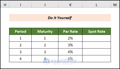
Practice Section
We have provided a Practice section like the one below in each sheet on the right side for you to practice.
Download the Practice Workbook
You may download the following Excel workbook and practice.
Related Articles
- How to Find Mean, Median, and Mode on Excel
- Comparison Among MAX vs MAXA vs LARGE and MIN vs MINA vs SMALL Functions in Excel
- How to Calculate Margin of Error in Excel
<< Go Back to Excel for Statistics | Learn Excel

