How to Scale Data from 1 to 10 in Excel (3 Quick Methods)

Sometimes when we work with data in Excel, we need the scaled value with respect to the range of data. It’s quite simple to scale data in Excel and it can be done following different methods. In this article, we will show 3 quick methods to Scale data from 1 to 10 in Excel.

How to Scale Data from 1 to 10 in Excel: 3 Quick Methods

Here, we will show 3 quick methods to scale data from 1 to 10. For the demonstration, we will take different ranges of data and scale them from 1 to 10. The scaled number will be different for different methods. Choose the method according to your need.

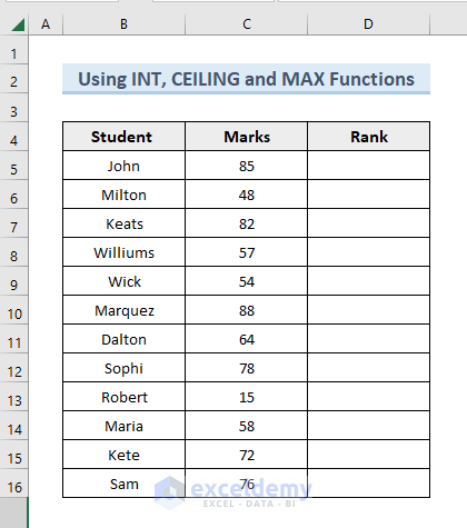
1. Use INT, CEILING and MAX Functions to Scale Data

In the first method, we have taken exam marks for a few students and we will scale the obtained marks on a scale of 10. We will use INT, CEILING and MAX functions of Excel for this method.

Follow the given steps for this method.

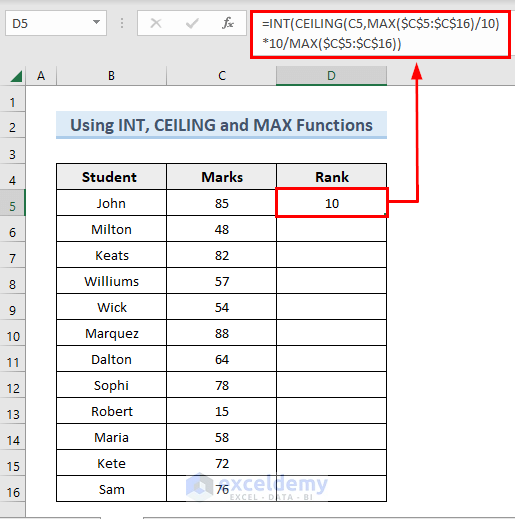
Firstly, write the following formula in Cell D5 to scale the data of Cell C5.

=INT(CEILING(C5,MAX($C$5:$C$16)/10)*10/MAX($C$5:$C$16))

Afterward, press Enter.
Consecutively, we will see the scaled value of Cell C5 in Cell D5.

🔎 How Does the Formula Work?

MAX($C$5:$C$16)/10: This part finds the maximum value of range $C$5:$C$16 and divides it by 10.
CEILING(C5,MAX($C$5:$C$16)/10: And here, the value of C5 is expressed as the immediate upper multiple of output from MAX($C$5:$C$16)/10 which is multiplied by 10 and divided by the maximum value of range $C$5:$C$16.
Lastly, the INT function takes the output as an argument and gives the respective integer value discarding the fractional part.

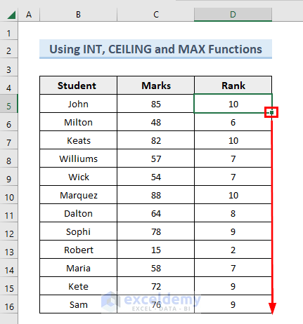
Further, use the Fill Handle to get the scaled values in the following cells.

Read More: How to Do Data Scaling in Excel

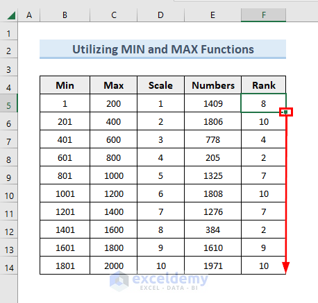
2. Utilizing MIN and MAX Functions for Scaling Data from 1 to 10

In this method, we will define the range value and their respective scaled value first. Then, we will compare any number with the range and find the right scaled value for that number by utilizing INDEX & MATCH functions. For demonstration, column Min & Max contains the range and column Scale contains their respective scaled value. Next, we will determine the scaled value in column Rank for Numbers column.

Follow the steps given for this method.

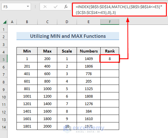
Firstly, write the following formula in Cell F5 to get the scaled value of Cell E5.

=INDEX($B$5:$D$14,MATCH(1,($B$5:$B$14<=E5)*($C$5:$C$14>=E5),0),3)

Then, press Enter and will see the scaled value in Cell F5.

🔎 How Does the Formula Work?

MATCH(1,($B$5:$B$14<=E5)*($C$5:$C$14>=E5),0): This part finds the row number of the range from Min & Max column where value of Cell E5 belongs.
The INDEX function takes the row number and gives the output from column 3 for that row number.

Finally, use the AutoFill feature to get the rest scaled value in the following cells.

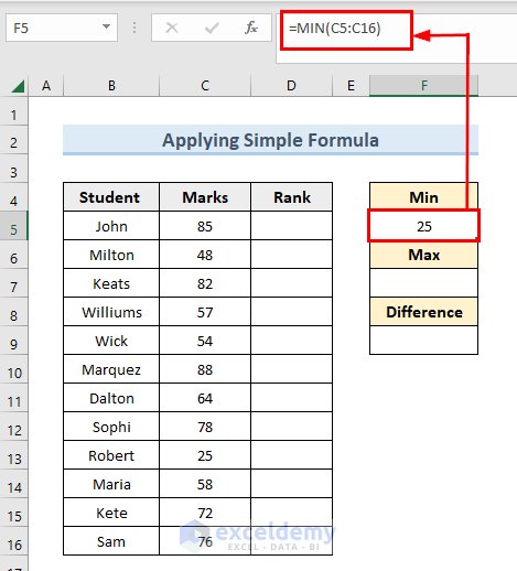
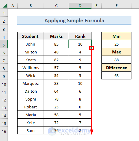
3. Scale Data from 1 to 10 Applying Simple Formula

We can use a comparatively simpler formula to get the scaled numbers. For this method, we have to determine the minimum and maximum values of the numbers to be scaled. Follow the given steps for this method to work.

Firstly, write the following formula in Cell F5 to get the minimum value of the range C5:C16.

=MIN(C5:C16)

Consecutively, press Enter.

Further, write the following formula in Cell F7 to get the maximum value of the range C5:C16.

=MAX(C5:C16)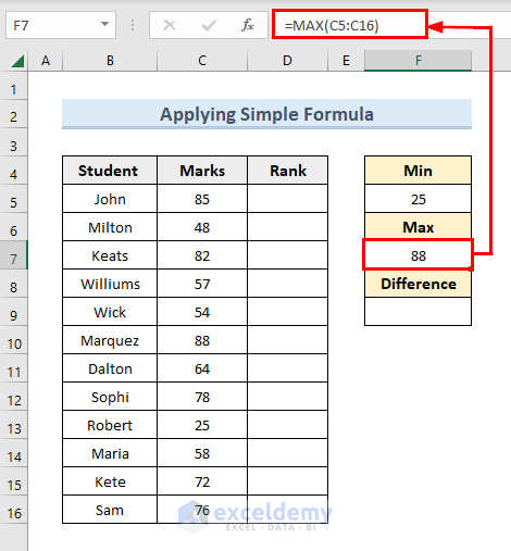

Afterward, determine the difference between the maximum value and minimum value in Cell F9 using the following formula.

=F7-F5

Later on, Press Enter.

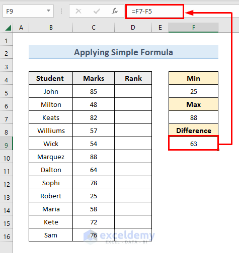
Now, we will use the previously determined maximum value and minimum value and their difference to determine the scaled value of the Marks column.

Firstly, write the following formula in Cell D5.

=ROUND((C5-$F$5)/$F$9*10,0)

Press Enter. Instantly, we will see the scaled value Cell C5 there.

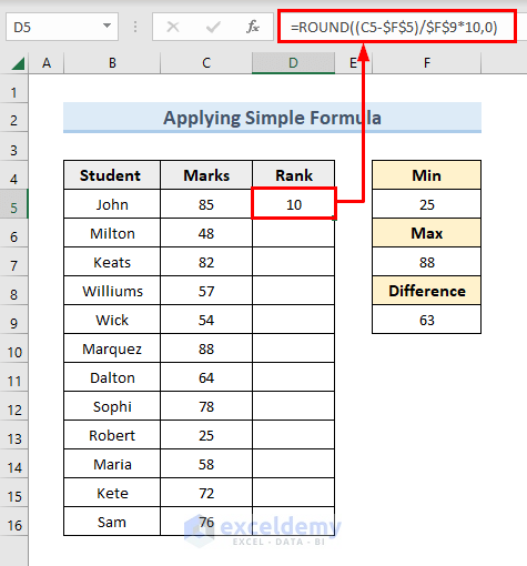
Note: We applied the formula Rank = (Original Value-Minimum value)/Difference of Maximum and Minimum Value*10. Later on, the ROUND function rounds the output number discarding the fractional value.

Finally, use the Fill Handle to copy the formula in the following cells and get the scaled value from range C5:C16.

Download Practice Workbook

You can download the practice workbook from here.

Scale Numbers from 1 to 10.xlsx

Conclusion

We have determined the 1 to 10 scaled value for different numbers following 3 quick methods. All the methods have different approaches so the scaled value differs. Follow the method that mostly fits your problem. If you have any queries or suggestions, let us know in the comment section.

<< Go Back to Scaling Formula in Excel | Excel for Statistics | Learn Excel

Get FREE Advanced Excel Exercises with Solutions!