Sometimes we have some blank cells in our dataset. When we plot them in an Excel chart, we can’t get the desired chart for these blank cells. In that case, we can ignore them by formulas. In this article, we will show how to ignore Excel chart blank cells with formulas effectively. I hope you find this article interesting.
How to Ignore Blank Cells with Formulas in Excel Chart: 2 Suitable Examples
To ignore Excel chart blank cells with formulas, we have two different examples through which you can have a clear idea of how to do it. In these two examples, we try to use the combinations of several functions. Finally, we will get our desired result. Both of these methods are fairly easy to use. Both of them will give us fruitful solutions.
1. Using Combined Formula
Our first method is based on using the combination of several functions. Here, we take a dataset that contains the date and profit. In that dataset, you will see several blank cells on both the date and profit columns. We will use the combination of IFERROR, INDEX, AGGREGATE, and ROW functions to eliminate the blank cells from the date column. We will use the INDEX and MATCH functions to eliminate the blank cells of the profit column. Then, we will create the line chart where all the blank cells will be ignored.
![]()
To understand the method clearly, let’s follow the steps.
Step 1: Find Date in Data Preparation Table
Here we can find the date in the data preparation table by using the INDEX function
- First, we want to prepare a data preparation table where we try to eliminate all the blank cells using the formulas.
- Then, select cell E6.
![]()
- Write down the following formula.
=INDEX($B$5:$B$14,1)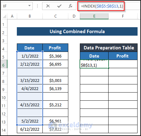
🔎 Breakdown of the Formula
INDEX($B$5:$B$14,1): The INDEX function returns a value of an array or table that is chosen by the given row and column. Here, we provide the array and row number. So, the INDEX function returns the value of the first row of the given array which is the first date.
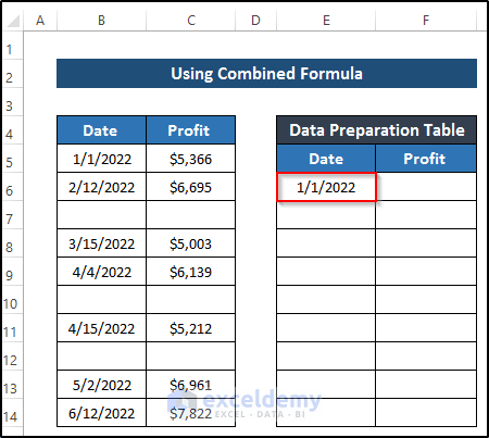
- Then, press Enter to apply the formula.
- It will show a number in cell E6 instead of a date.
![]()
- To convert it into a date, select cell E6.
- Then, go to the Home tab in the ribbon.
- From the Number group, click on the downward arrow of the Number Format box.
- Then, select the Short Date option.
![]()
- As a result, it will change the number and convert it into the required date.
Step 2: Add Serial to Data Preparation Table
In this step, we want to add a new column known as Serial. We want to use that serial number as a reference in the formula
- Create a Serial column from 1 to 10.
![]()
- Then, change the formula of cell E6.
- Replace 1 with cell G6.
- Then, the formula of cell E6 will be like the following.
=INDEX($B$5:$B$14,G6)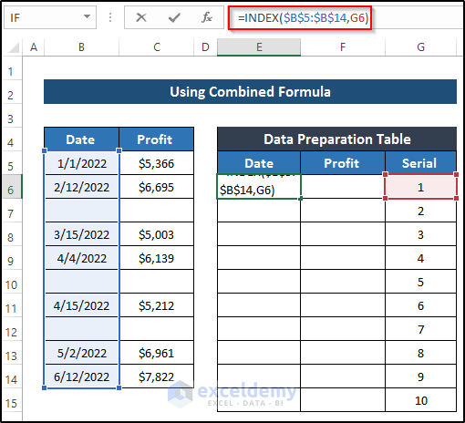
- Press Enter to apply the formula.
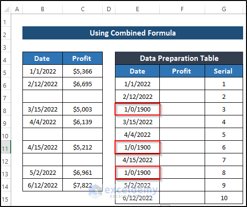
- Then, drag the Fill Handle icon down the column.
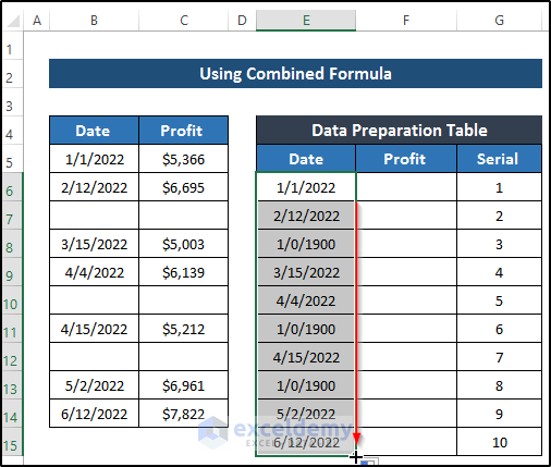
- As a result, you will see the cells E8, E11, and E13 have date values that are not real dates. Because we don’t have dates in cells B7, B10, and B12.
Step 3: Add Row Number in Data Preparation Table
In this step, we want to add another column known as row number. Here, we will use the combination of AGGREGATE and ROW Functions.
- First, we need to add another column known as Row Number.
- Select cell H6.
![]()
- Then, write down the following formula.
=AGGREGATE(15,3,ROW($B$5:$B$14),G6)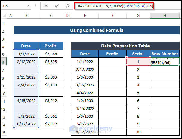
🔎 Breakdown of the Formula
AGGREGATE(15,3,ROW($B$5:$B$14),G6): Here, the AGGREGATE function has several options to ignore blank rows with error values. 15 denotes SMALL function number, 3 denotes ignore hidden rows, error values, nested SUBTOTAL, and AGGREGATE Functions. The AGGREGATE function uses this function and options in the given array and returns a number value.
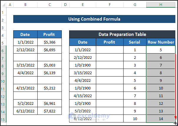
- Press Enter to apply the formula.
![]()
- Then, drag the Fill Handle icon down the column.
- As we have blank cells in the dataset, we want to skip those rows in the Row Number column. That’s why we need to do some modifications to our formula.
- First, select cell H6.
- Then, write down the following formula instead of the previous one.
=AGGREGATE(15,3,ROW($B$5:$B$14)/($B$5:$B$14<>""),G6)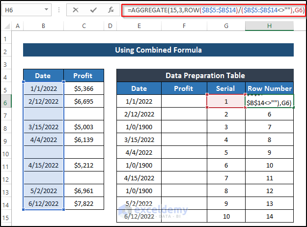
🔎 Breakdown of the Formula
AGGREGATE(15,3,ROW($B$5:$B$14)/($B$5:$B$14<>””),G6): Here, the ROW function returns the array for the AGGREGATE function. Then, the AGGREGATE function uses the function and options in the given array. Finally, it returns a number value.
- Then, drag the Fill Handle icon down the column.

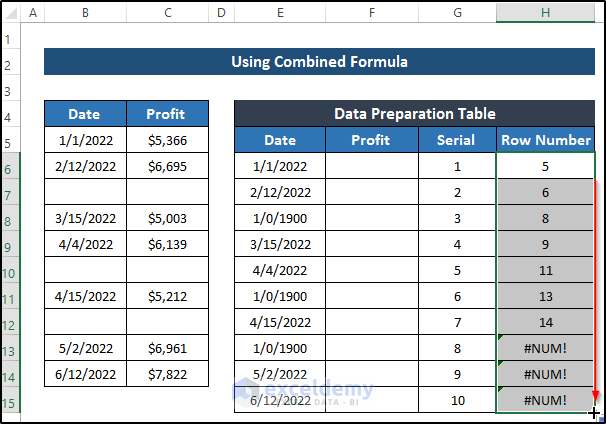
- After that, we will use the ROWS Function to remove the need for the Serial We want to delete the serial column from the data preparation table, that’s why we want to do this.
- Select cell H6.
- Then, delete the previous formula and write down the following formula.
=AGGREGATE(15,3,ROW($B$5:$B$14)/($B$5:$B$14<>""),ROWS($B$5:B5))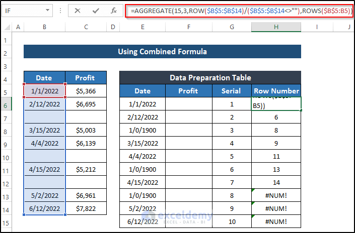
- Then, press Enter to apply the formula.
- After that, drag the Fill Handle icon down the column.
- Here, the row number starts from 5. But we want to start row number from 1.
- In that case, you have to do some more modifications in cell H6.
- Then, select cell H6.
- After that, write down the following formula instead of the previous one.
=AGGREGATE(15,3,ROW($B$5:$B$14)-ROW($B$4)/($B$5:$B$14<>""),ROWS($B$5:B5))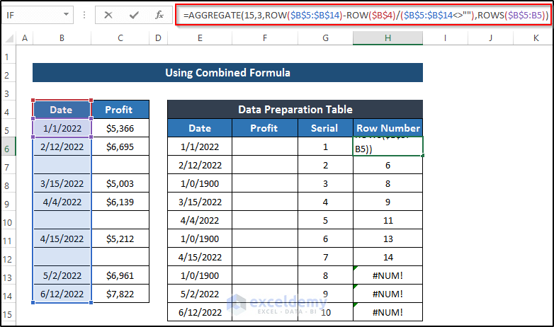
🔎 Breakdown of the Formula
AGGREGATE(15,3,ROW($B$5:$B$14)-ROW($B$4)/($B$5:$B$14<>””),ROWS($B$5:B5)): Here, we want to start row number from 1. The AGGREGATE function has several options to ignore blank rows with error values. 15 denotes SMALL function number, 3 denotes ignore hidden rows, error values, nested SUBTOTAL, and AGGREGATE Functions.
ROW($B$5:$B$14)-ROW($B$4)/($B$5:$B$14<>””): It denotes that if there is a blank cell, it will skip it and go to the next. The AGGREGATE function uses this array and finally returns the row number from 1.
- Then, press Enter to apply the formula.
- After that, drag the Fill Handle icon down the column.
![]()
- Now, we want to copy the formula from cell H6 and paste it into cell E6.
- The Formula in cell E6 is
=INDEX($B$5:$B$14,G6)In this formula, we only replace the G6 and put the formula of cell H6.
- When we replace this in cell E6, then the whole formula will be like the following.
=INDEX($B$5:$B$14,AGGREGATE(15,3,ROW($B$5:$B$14)-ROW($B$4)/($B$5:$B$14<>""),ROWS($B$5:B5)))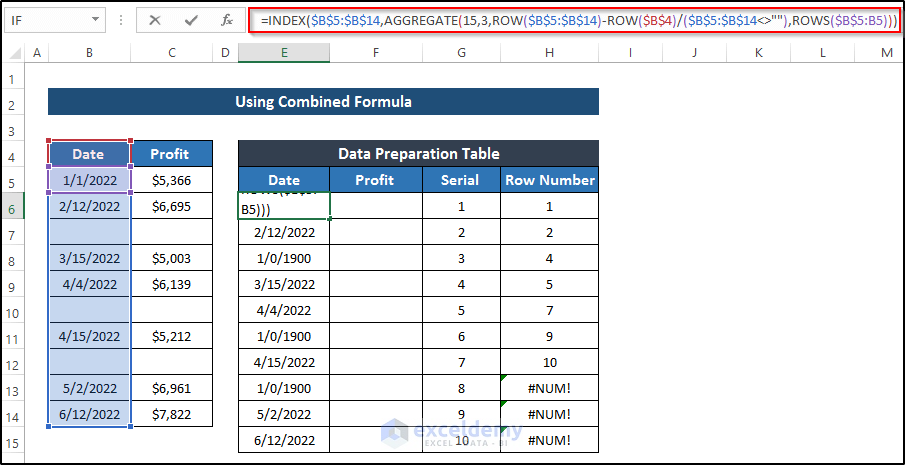
🔎 Breakdown of the Formula
INDEX($B$5:$B$14,AGGREGATE(15,3,ROW($B$5:$B$14)-ROW($B$4)/($B$5:$B$14<>””),ROWS($B$5:B5))): Here, the AGGREGATE function provides the row number. The INDEX function uses that row number in the given array and returns the required date.
- We need to use the IFERROR function along with this formula to eliminate any type of error.
- Then, write down the following formula in cell E6.
=IFERROR(INDEX($B$5:$B$14,AGGREGATE(15,3,ROW($B$5:$B$14)-ROW($B$4)/($B$5:$B$14<>""),ROWS($B$5:B5))),"")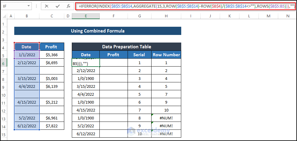
🔎 Breakdown of the Formula
IFERROR(INDEX($B$5:$B$14,AGGREGATE(15,3,ROW($B$5:$B$14)-ROW($B$4)/($B$5:$B$14<>””),ROWS($B$5:B5))),””): Here, the IFERROR function denotes if there is an error, it will return blank. Otherwise, it will return the required date. As cell B5 doesn’t contain a blank, the IFERROR function will return the INDEX function value.
- Then, drag the Fill Handle icon down the cell.
![]()
- After that, delete both Serial and Row Number Because there is no need to keep them.
Step 4: Find Profit in Data Preparation Table
we need to complete the profit column by using the INDEX and MATCH functions.
- First, select cell F6.
- Write down the following formula.
=INDEX($C$5:$C$14,MATCH(E6,$B$5:$B$14,0))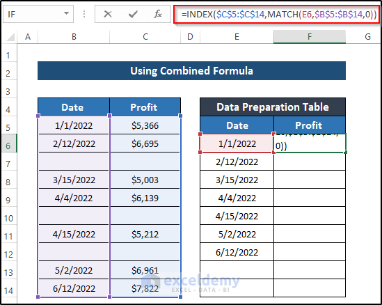
- Then, press Enter to apply the formula.
![]()
- After that, drag the Fill Handle icon down the column.

Step 5: Establish Line Chart Using Data Preparation Table
In this step, we will prepare a line chart using the data preparation table.
- First, select the range of cells E6 to F12.
![]()
- Then, go to the Insert tab in the ribbon.
- From the Charts group, select Recommended Charts option.
![]()
- Then, the Insert Chart dialog box will appear.
- Select Line Chart from there.
- Finally, click on OK.
![]()
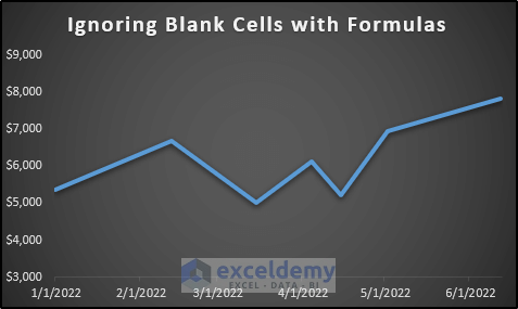
- After modifying the chart style, we will get the following line chart where the blank cells are ignored. See the screenshot.
- To modify the horizontal axis, right-click on the axis.
- From the Context Menu, select Format Axis.
![]()
- Then, the Format Axis dialog box will appear.
- Select the Text axis from the Axis Options section.
![]()
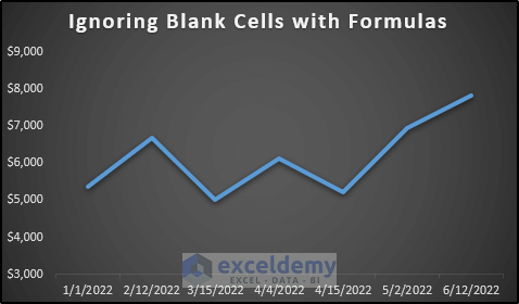
- Finally, we get our desired line chart. See the screenshot.
Read More: How to Skip Data Points in an Excel Graph
2. Combining IF, ISBLANK and NA Functions
Our second method is based on the combination of IF, ISBLANK, and NA Functions. In this method. We want to replace the blank cells with the #NA. Because of this, the Excel chart will ignore blank cells. To show the method correctly, we take a dataset that contains months and their corresponding profit value.
![]()
To understand the method clearly, you need to follow the steps.
Steps
- First, select the range of cells B4 to C16.
![]()
- Then, go to the Insert tab in the ribbon.
- From the Charts group, select Recommended Charts option.
![]()
- Then, the Insert Chart dialog box will appear.
- Select Line Chart from there.
- Finally, click on OK.
![]()
- After Modifying the chart style and axis, we get the following result.
- As we don’t use any formula in the blank cells, it puts blank cells also in the Excel chart.
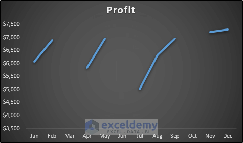
- To solve the problem, we need to create another column named Modified Profit.
- First, select cell D5.
![]()
- Then, write down the following formula in the formula box.
=IF(ISBLANK(C5),NA(),C5)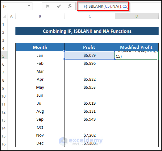
🔎 Breakdown of the Formula
IF(ISBLANK(C5),NA(),C5): Here, the ISBLANK function checks cell C5 whether it is blank or not. If it is blank, then the IF function returns the NA function otherwise returns cell C5.
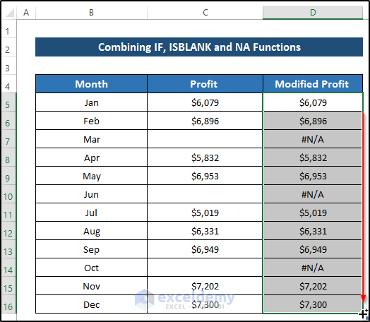
- After that, press Enter to apply the formula.
![]()
- Then, drag the Fill Handle icon down the column. Here, you will see #NA replaces all the blank cells.
- Now, select the range of cells D5 to D16.
![]()
- Then, go to the Insert tab in the ribbon.
- From the Charts group, select Recommended Charts option.
![]()
- Then, the Insert Chart dialog box will appear.
- Select Line Chart from there.
- Finally, click on OK.
![]()
- Here we have our Line chart where all the blank cells are ignored.

- Then, to modify the horizontal axis of the chart, right-click on the chart.
- From the Context Menu, select the Select Data option.
![]()
- Then, the Select Data Souce dialog box will appear.
- Click on the Horizontal Axis Labels.
![]()
- Then, select the Month column in the Axis Labels dialog box.
- Finally, click on OK.
![]()
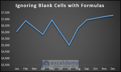
- Finally, after modifying the chart style, we get our desired chart where the blank cells are ignored. See the screenshot.
Read More: How to Limit Data Range in Excel Chart
Download Practice Workbook
Download the practice workbook below.
Conclusion
We have shown two examples to ignore Excel chart blank cells with formulas. In this article, we basically utilize several effective Excel functions and their combination. By combining them neatly, we found our desired result. I hope we covered all possible areas about ignoring blank cells with formulas.
Related Articles
- How to Change Chart Data Range in Excel
- How to Edit Data Table in Excel Chart
- How to Change Data Source in Excel Chart
- How to Edit Chart Data in Excel
- How to Change X-Axis Values in Excel
- How to Change Chart Data Range Automatically in Excel
- How to Sort Data in Excel Chart
- How to Group Data in Excel Chart
- How to Remove One Data Point from Excel Chart
- How to Hide Chart Data in Excel
<< Go Back to Data for Excel Charts | Excel Charts | Learn Excel
Get FREE Advanced Excel Exercises with Solutions!
