How to Hide Chart Data in Excel – 6 Steps

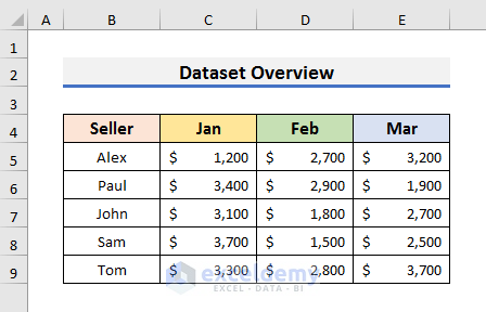
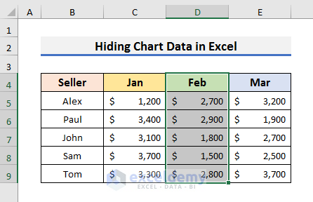
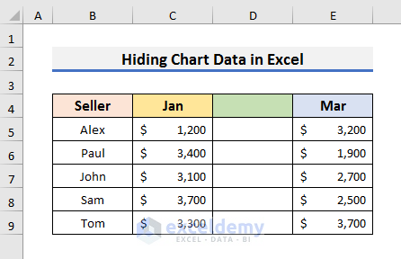
The sample dataset contains information on sales amounts in three months. To hide the sales amount for February:

STEP 1 – Plotting a Chart in Excel

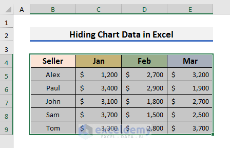
• Select any cell in the dataset and press Ctrl + A to select all used cells.

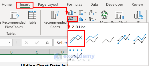
• Go to the Insert tab and select Insert Line.
• Select Line.

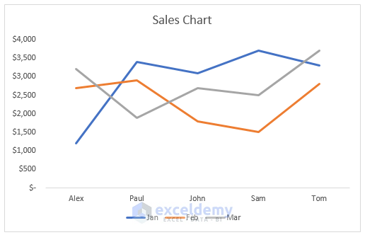
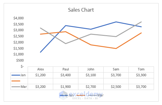
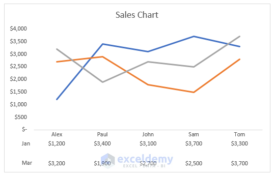
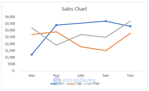
You will see a line chart.

Read More: How to Edit Chart Data in Excel

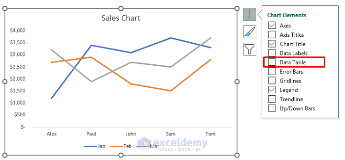
STEP 2 – Inserting a Chart Data Table

• Select the chart. A plus (+) icon will appear on the top right side of the chart.
• Click the plus (+) icon.
• Check Data Table.

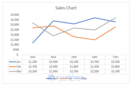
You can see the dataset inside the chart.

Read More: How to Change Data Source in Excel Chart

STEP 3 – Hiding Chart Data in Excel

• Select D4:D9.

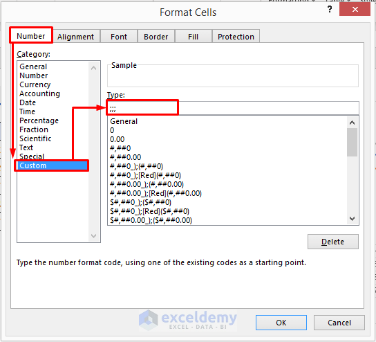
• Press Ctrl + 1 to open the Format Cells dialog box.
• Click the Number tab and select Custom.
• Enter three semi–colons (;;;) in Type.
• Click OK.

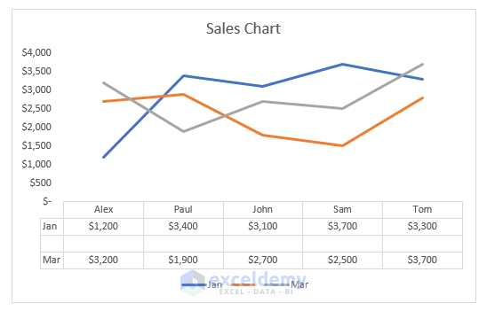
You will hide the data for February in the dataset.

And also in the Data Table.

STEP 4 – Removing Legend Keys to Hide Chart Data

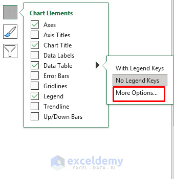
• To remove Legend Keys, select the chart and click the plus (+) icon.
• Select the arrow to see the options.
• Select No Legend Keys.

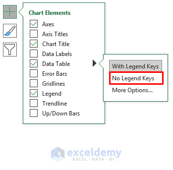
• No Legend Keys for February will be displayed.

Read More: How to Remove One Data Point from Excel Chart

STEP 5 – Remove the Chart Data Table Borders

• Select the chart and click the plus (+) icon.
• Select the arrow to see the options.
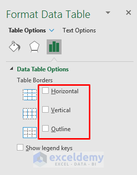
• Select More Options to open Format Data Table.

• Uncheck Table Borders in Data Table Options.

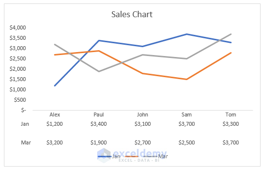
This is the output.

STEP 6  – Deleting Chart Legends

• Click the Legends and press Delete.

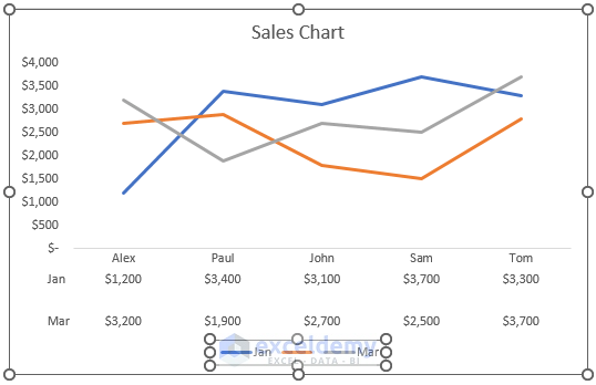
This is the output.

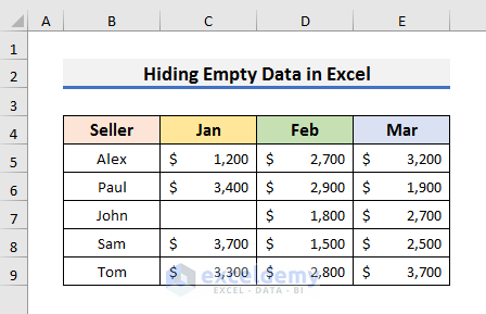
How to Hide Empty Data in an Excel Chart

There is empty data in C7.

STEPS:

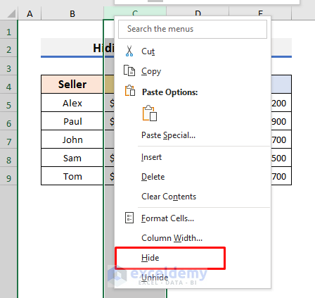
• Select the column with the empty cell.
• Right–click the column index.
• Select Hide.

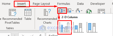
• Select all cells in the dataset.

• Go to the Insert tab and select Insert Column.
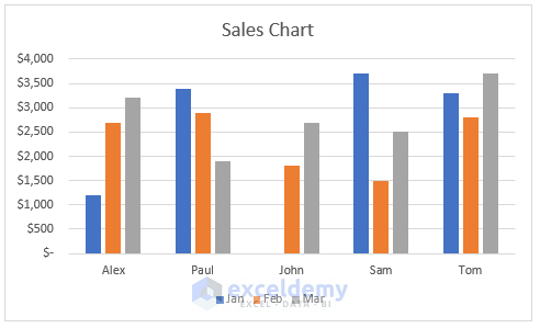
• Choose Clustered Column.

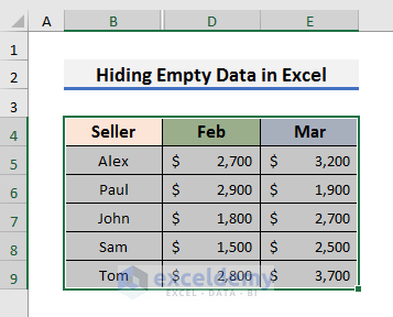
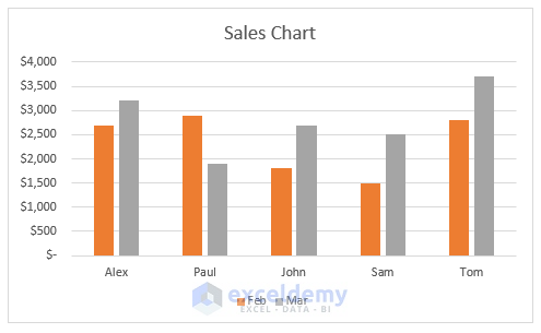
You will see the chart. Data for January is hidden.

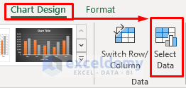
• Select the chart and go to the Chart Design tab.
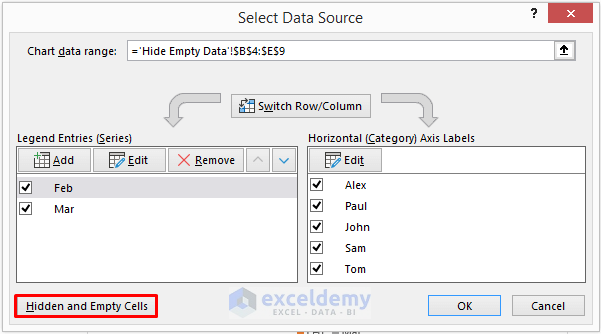
• Click Select Data to open the Select Data Source dialog box.

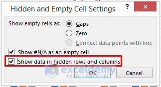
• Click Hidden and Empty Cells.

• Check Show data in hidden rows and columns in Hidden and Empty Cell Settings.
• Click OK.

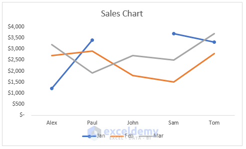
You will see the data for January.

This is the output. There is a disconnected line for January because of the empty cell.

• Select ‘Connect data points with line’ in Hidden and Empty Cell Settings.

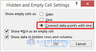
This is the output.

Download Practice Workbook

Download the practice book.

Related Articles

• How to Change Chart Data Range in Excel
• How to Edit Data Table in Excel Chart
• How to Change X-Axis Values in Excel
• How to Change Chart Data Range Automatically in Excel
• How to Sort Data in Excel Chart
• How to Group Data in Excel Chart
• How to Limit Data Range in Excel Chart
• How to Skip Data Points in an Excel Graph

<< Go Back to Data for Excel Charts | Excel Charts | Learn Excel