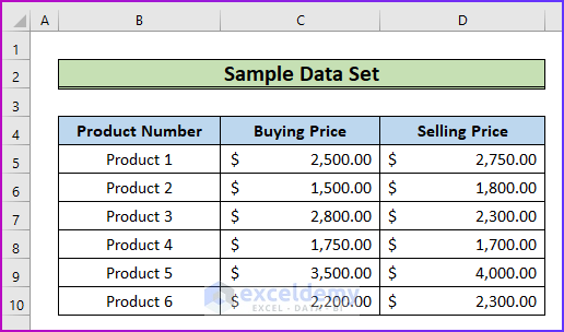
This is the sample dataset.
Step 1 – Use a Formula to Calculate the Output
- Insert a new column to show the profit.
- Enter the following formula in E5.
=IF(C5<D5,D5-C5,"")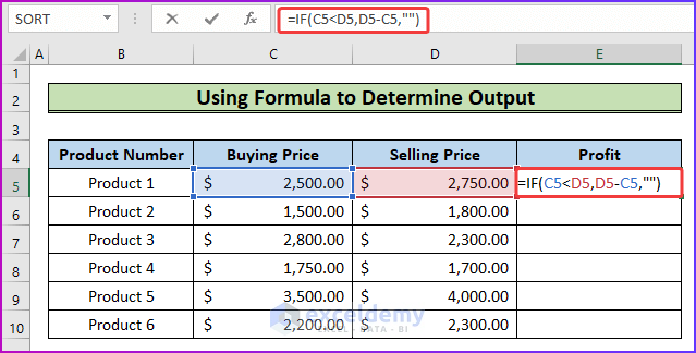
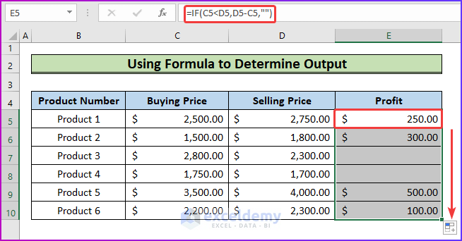
- Press Enter to see the profit of the first product.
- Drag down the Fill Handle to see the result in the rest of the cells.
Read More: How to Limit Data Range in Excel Chart
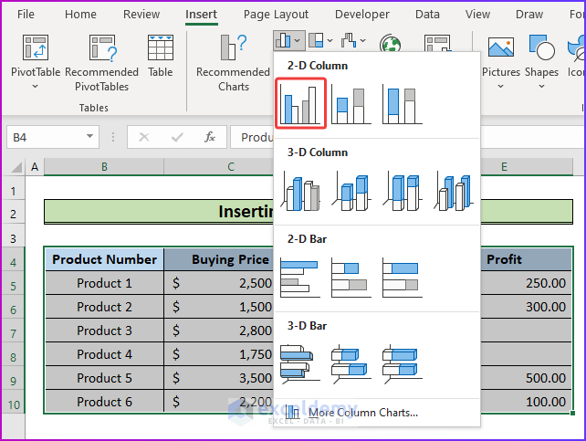
Step 2 – Insert a Column Chart
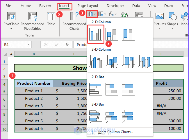
- Select B4:E10.
- Go to the Insert tab.
- In Charts, select Insert Column or Bar Chart.
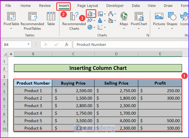
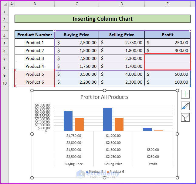
- Choose Clustered Column.
The chart is displayed. It does not contain all data points and only shows data after product 4.
Step 3 – Modify the Formula
To skip these data points, modify the formula (enter #N/A as a value if the logical test of the formula is false):
- Enter the formula in E5.
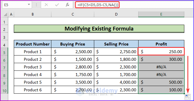
=IF(C5<D5,D5-C5,NA())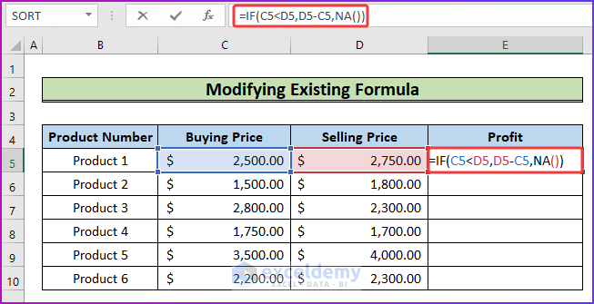
- Press Enter and drag down the Fill Handle.
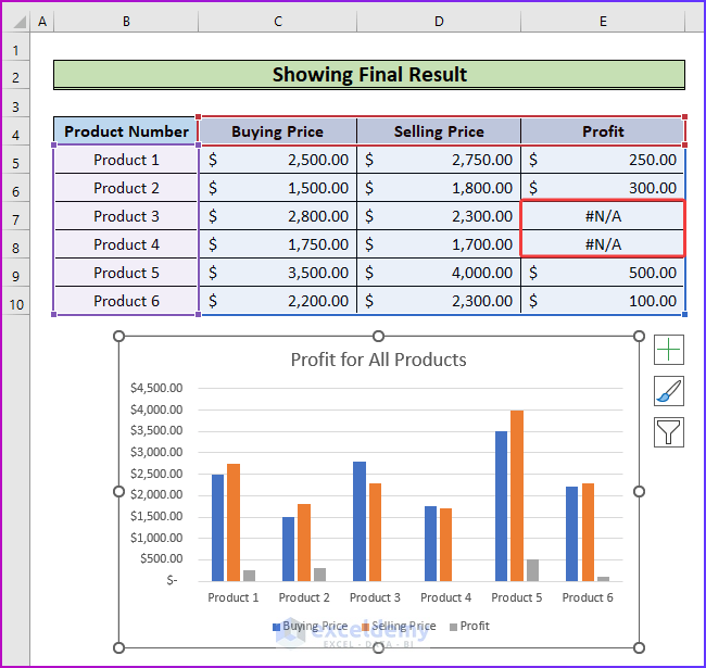
Cells with products whose selling prices are less than the buying price will show #N/A, instead of empty cells in the Profit column.
Read More: How to Edit Chart Data in Excel
Step 4 – Show the Final Result
- Select B5:E10 and insert the column chart (as described in Step 2).
The data points of Product 3 and 4 were skipped and the graph starts from product 1.
Download Practice Workbook
Download the free Excel workbook.
Related Articles
- How to Change Chart Data Range in Excel
- How to Edit Data Table in Excel Chart
- How to Change Data Source in Excel Chart
- How to Change X-Axis Values in Excel
- How to Change Chart Data Range Automatically in Excel
- How to Sort Data in Excel Chart
- How to Group Data in Excel Chart
- How to Remove One Data Point from Excel Chart
- How to Hide Chart Data in Excel
<< Go Back to Data for Excel Charts | Excel Charts | Learn Excel
Get FREE Advanced Excel Exercises with Solutions!

Thanks but this won’t work because I don’t want the table changed. I repeat the headings on my chart every month because they are needed. The problem is when I try to make a table over several years of data, the headings are getting treated as zeros in my graph. I am looking for a way to exclude the headings because they aren’t actually data points at all.
I was hoping for a formula to exclude text, non-numerical input, or an IF function to exclude zeros. I did try setting the y-axis minimum to 10 since my real data points are all around 30-40, but the line on my scatter plot still tries to connect to them. I will try just giving up on the line, but I did actually want it.
Hello L. O.
Thanks for reaching out and sharing your problem. You are facing difficulties with including a heading in a chart, and those headings affect the graph’s appearance.
As the headings are treated as zeros, you can exclude them from the data by combining the IF, ISNUMBER and NA functions. The formula structure can be like the following:
This formula checks if the value in cell A2 is a number. If it is, it includes the value. Otherwise, it returns #N/A. The #N/A values will be ignored in the chart, and the line won’t connect to them.
Instead of a scatter plot, you might consider using a line chart or other chart types that suit your needs better. Line charts, for example, automatically ignore #N/A values and don’t connect them.
Hopefully, the ideas will help you to overcome your situation. Good luck!
Regards
Lutfor Rahman Shimanto
ExcelDemy