How to Format a Data Table in an Excel Chart – 4 Methods

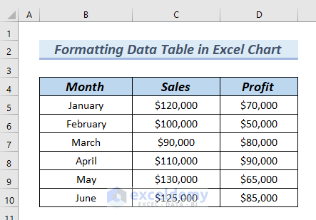
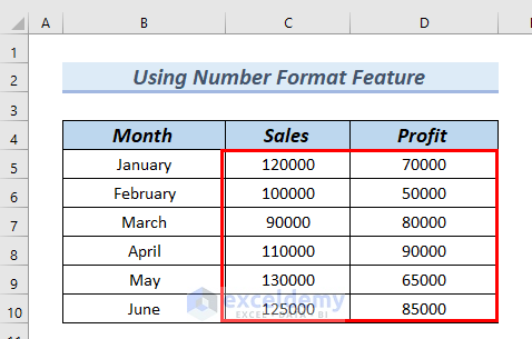
The following dataset contains Month, Sales, and Profit columns. To insert a Column chart:

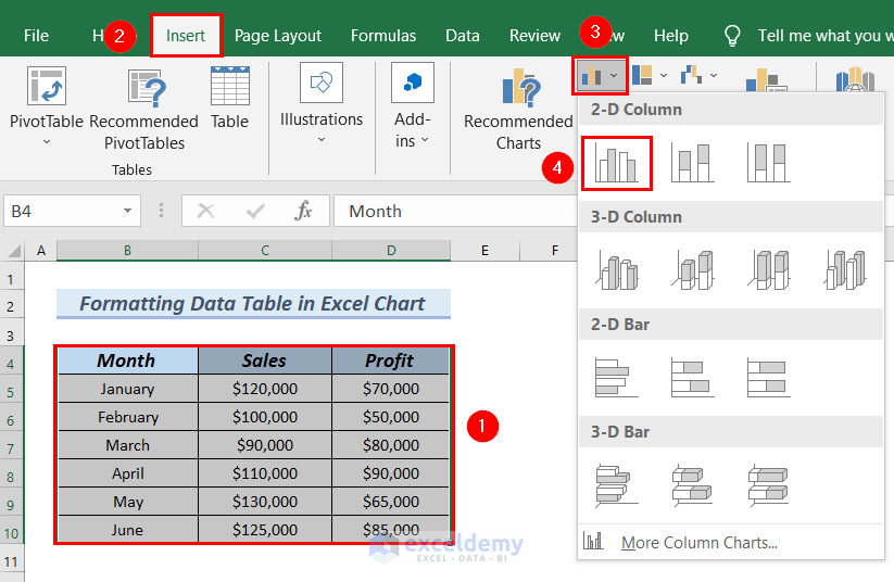
• Select the entire dataset: B4:D10.
• Go to the Insert tab.
• In Insert Column or Bar Chart >> select 2D Clustered Column chart.

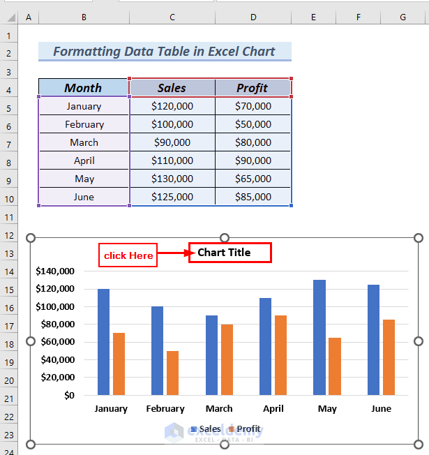
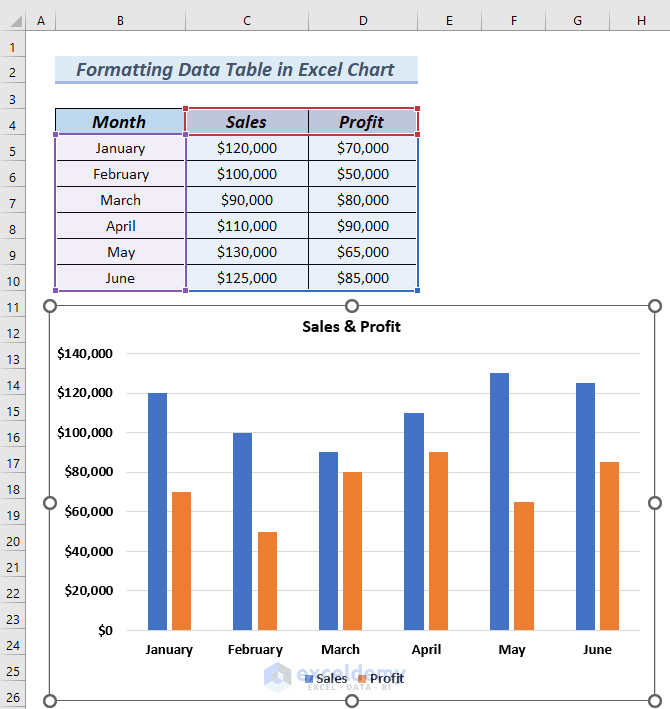
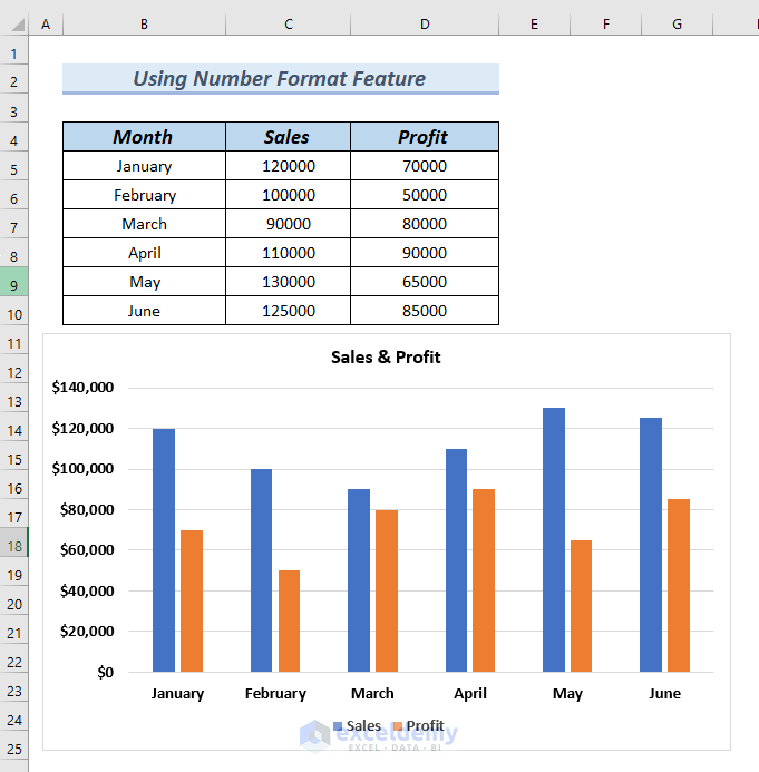
The Column chart is displayed.

• Click the Chart Title to edit it.

Method 1 – Using the Number Format Feature to Format a Data Table in an Excel Chart

To change the format of the chart Data Table by changing the format of the source Dataset:

Step 1: Inserting a Column Chart and Adding a Data Table

• Insert a Column chart by following the steps described above.

Add a Data Table to the chart.

• Click Chart Elements.
• Check Data Table.

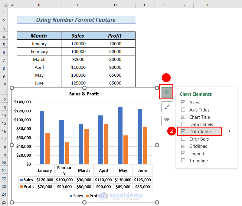
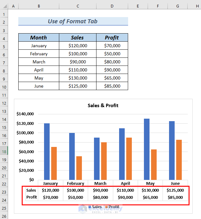
A Column chart and a Data Table are displayed.

The Sales and Profit values are in General number format.

Step 2: Applying the Currency Number Format to Chart a Data Table

• Select the values in the Sales and Profit columns: C5:D10.
• Go to the Home tab >> click Number Format.
• Select Currency.

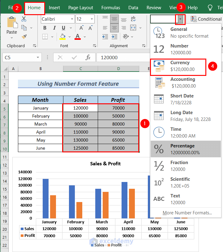
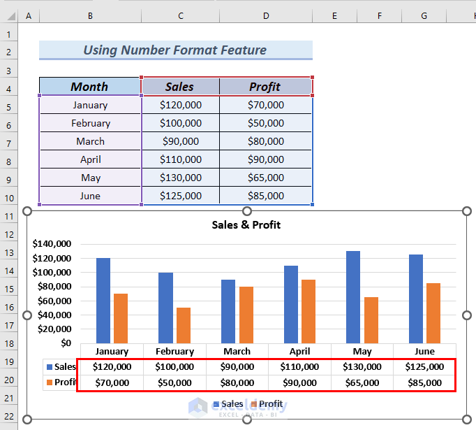
The Sales and Profit columns are in Currency number format.

The chart Data Table is also in Currency number format.

Read More: How to Add Data Table in an Excel Chart

Method 2 – Using the Format Tab to Format a Data Table in an Excel Chart

Steps:

• Insert a Column chart by following the steps described above.
• Add the chart Data Table by following step1 of Method-1.

A Column chart with the chart DataTable will be displayed.

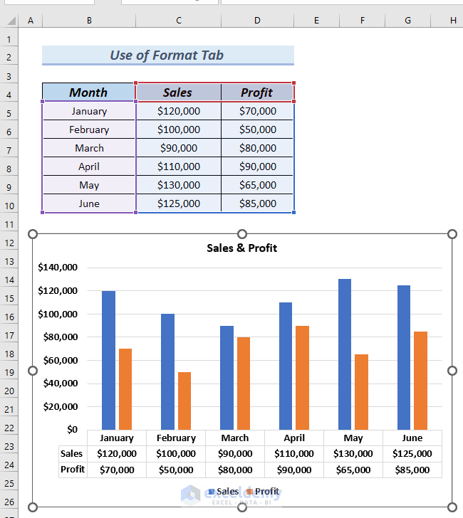
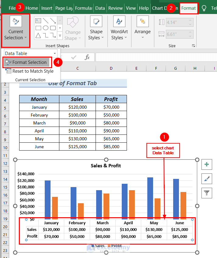
Format the chart Data Table so that it has no Horizontal outline.

• Select the chart Data Table >> go to the Format tab.
• In Current Selection >> select Format Selection.

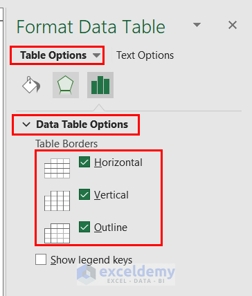
• In the Format Data Table dialog box, select Data Table Options.
• All Table Borders are checked.

• Uncheck Horizontal.

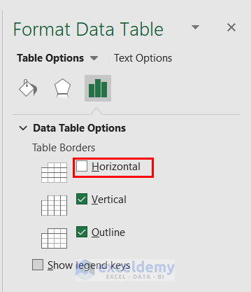
The chart Data Table has no Horizontal border.

Method 3 – Using the Chart Design Tab in Excel

Steps:

• Insert a Column chart by following the steps described above.

You will see a Column chart.

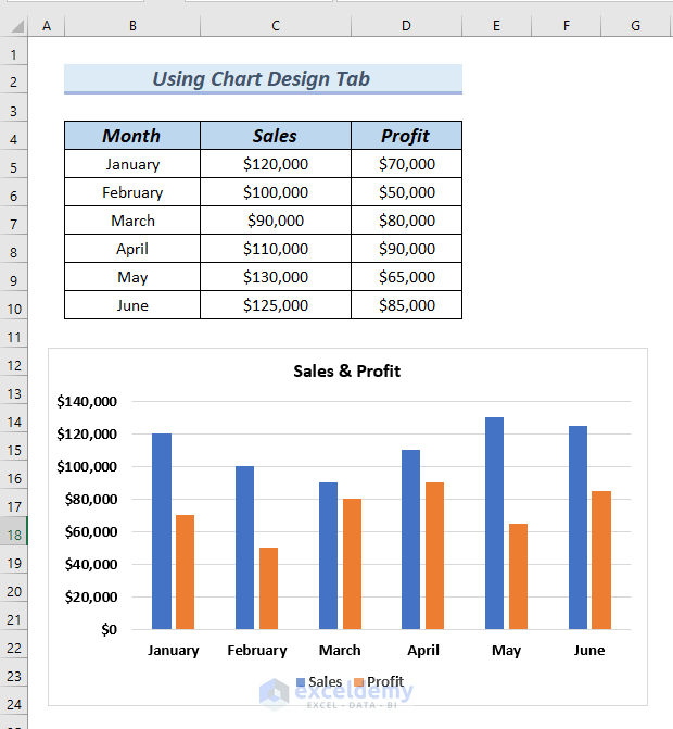
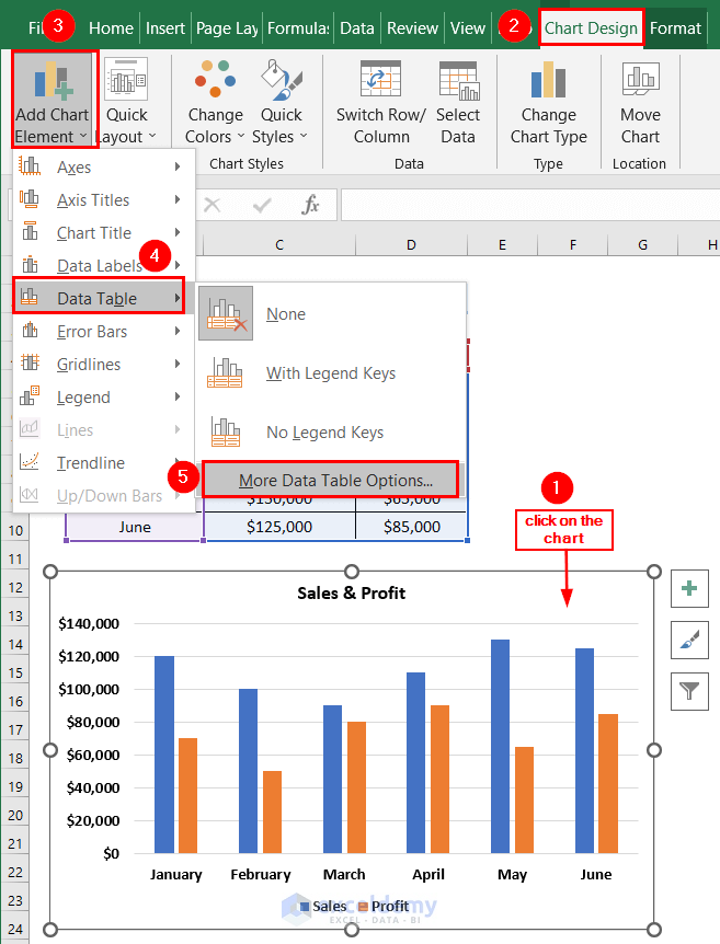
• Go to the Chart Design tab.
• In Add Chart Element >> select Data Table.
• Select More Data Table Options.

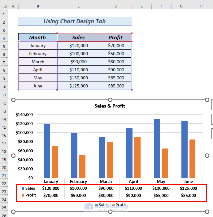
A chart Data Table is displayed.

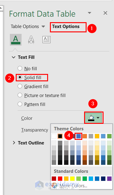
In the Format Data Table dialog box:

• Click Text Options.
• Click Solid Fill >> click the icon of the Color box.
• Select a color. Here, Blue.

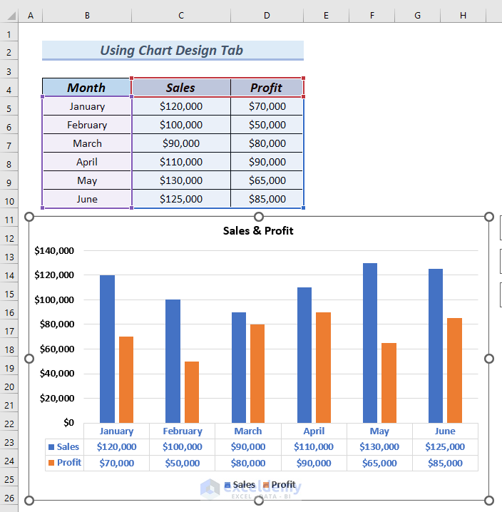
You can see the chart Data Table in Blue.

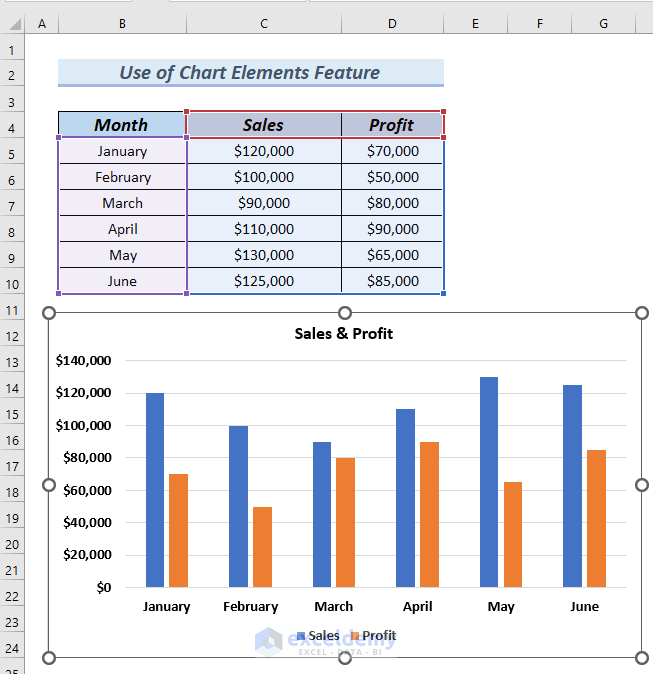
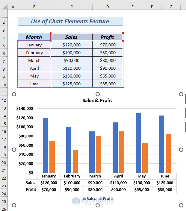
Method 4 – Using the Chart Elements Feature to Format a Data Table in an Excel Chart

Steps:

• Insert a Column chart by following the steps described above.

You will see a Column chart.

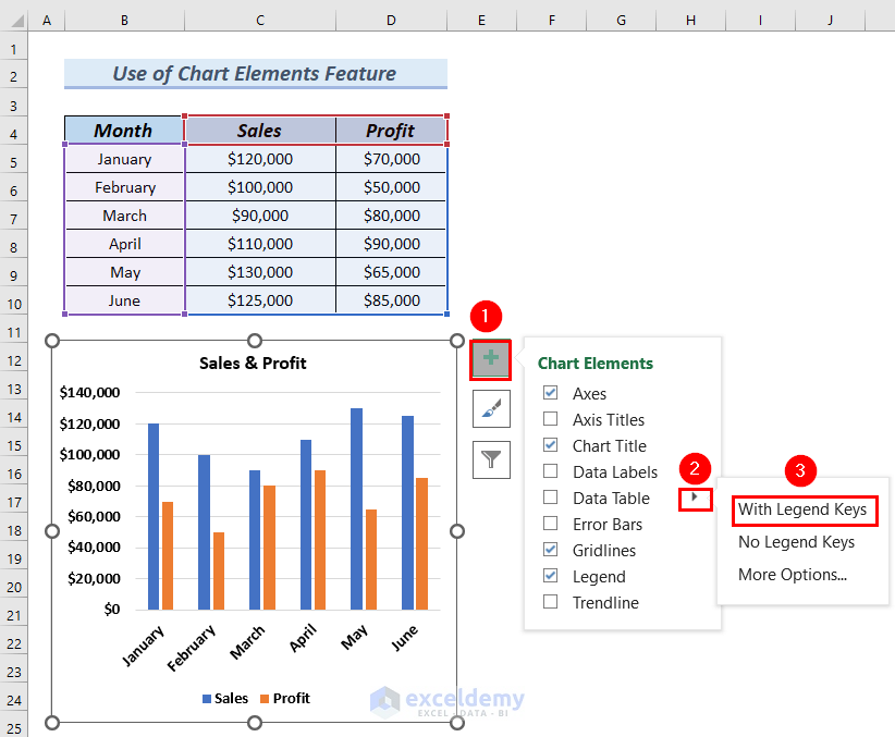
To add a chart Data Table with legends keys:

• Click Chart Elements >> click the rightward arrow in Data Table.
• Select With Legend Keys.

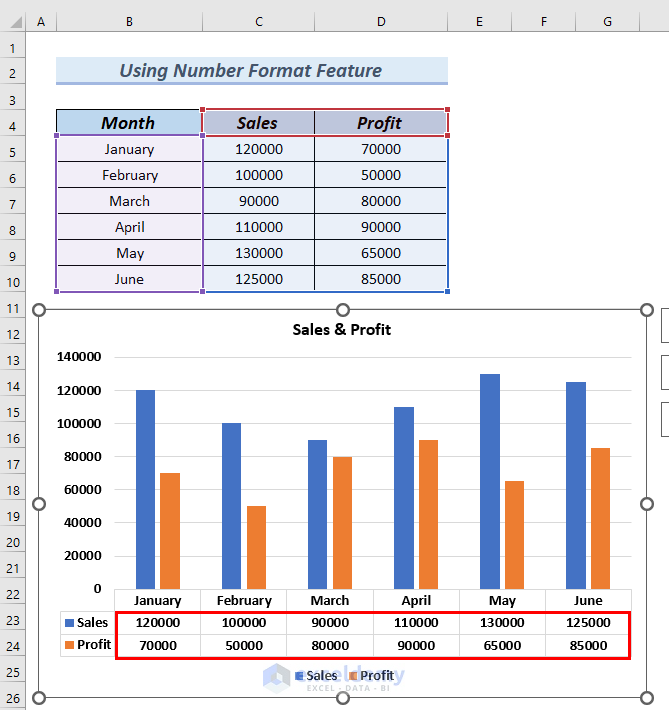
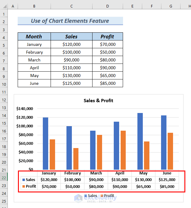
You will see the chart Data Table with Legend keys.

To add a chart Data Table without legend keys:

• Click Chart Elements >> click the rightward arrow in Data Table.
• Select No Legend Keys.

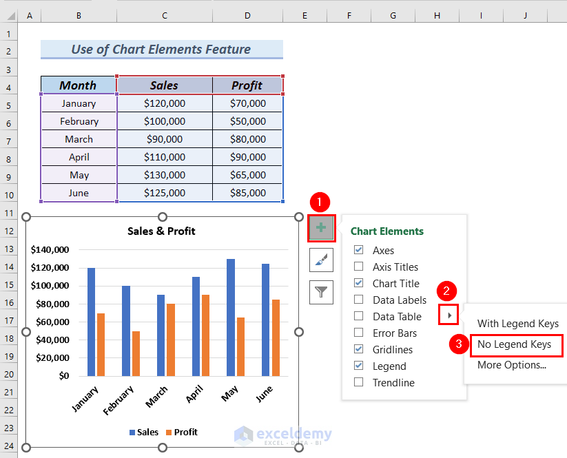
You will see the chart Data Table with no Legend Keys.

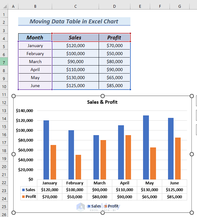
How to Move a Data Table in an Excel Chart

• Insert a Column chart by following the steps described above.
• Add the chart Data Table by following step 1 in Method 1.

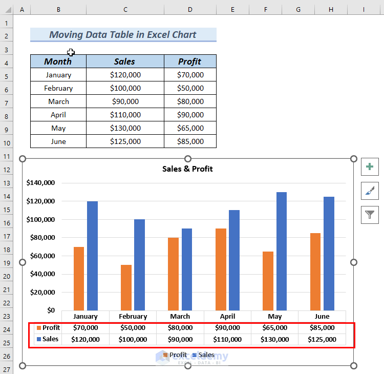
You will see a Column chart with the chart DataTable.

The Sales is above the Profit.

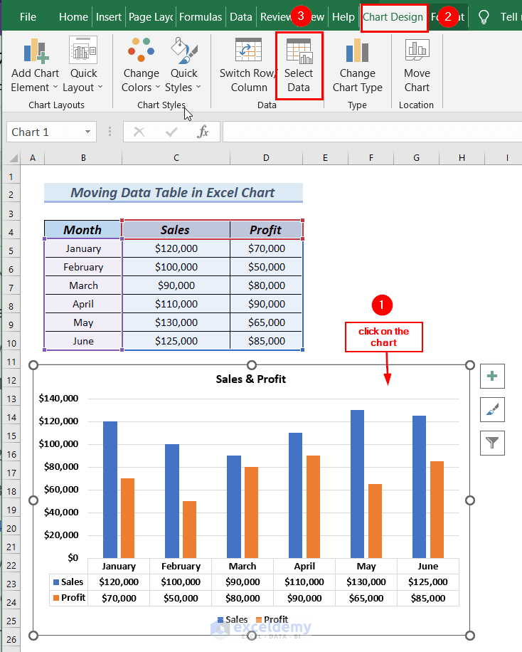
To change the order:

• Click the chart >> go to the Chart Design tab.
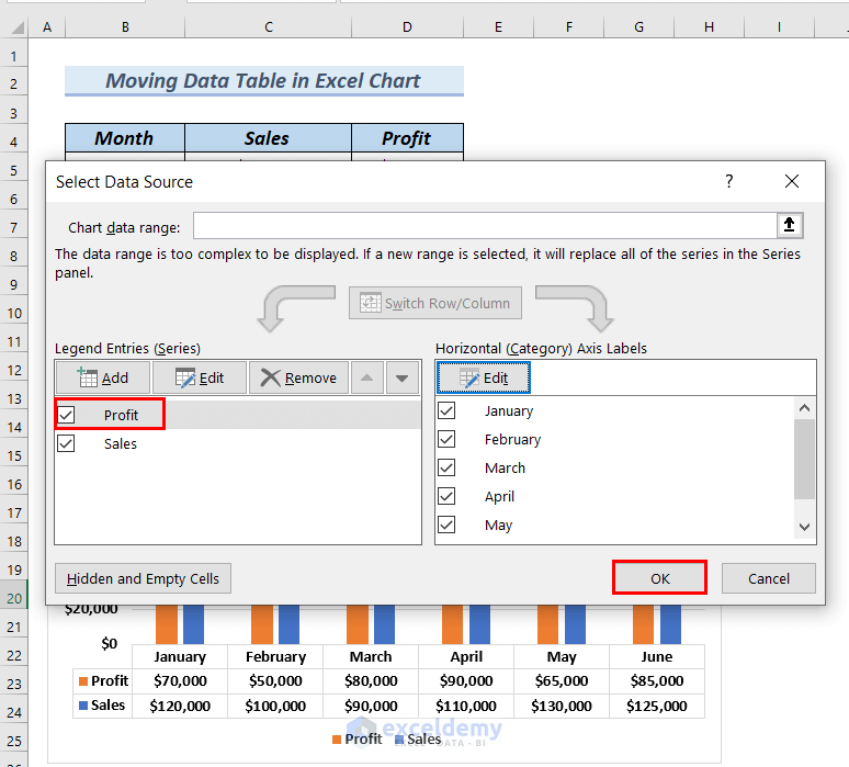
• In Data >> choose Select Data.

In the Select Data Source dialog box:

• Click Profit >> select the upward arrow as shown below.

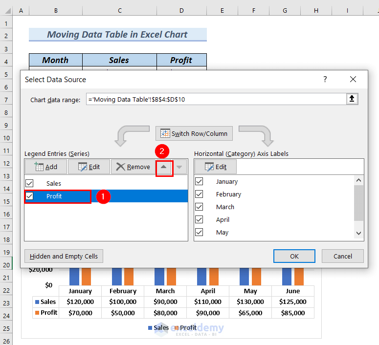
Profit is now above Sales.

• Click OK.

This is the output.

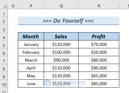
Practice Section

Download the Excel file to practice.

Download Practice Workbook

Download the Excel file and practice.

Related Articles

• How to Select Data for a Chart in Excel
• Selecting Data in Different Columns for an Excel Chart
• How to Expand Chart Data Range in Excel
• How to Add Data to an Existing Chart in Excel
• How to Add Data Points to an Existing Graph in Excel
• How to Create Excel Chart Using Data Range Based on Cell Value
• How to Get Data Points from a Graph in Excel

<< Go Back to Data for Excel Charts | Excel Charts | Learn Excel