How to Expand Chart Data Range in Excel: 5 Methods

Method 1 – Expand Chart Data from Chart Design Options

Steps:

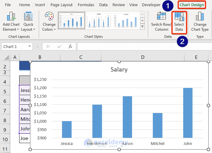
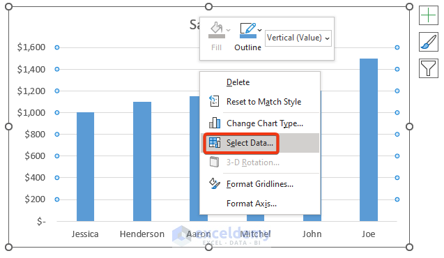
• Click the Chart. The Chart Design shows now.
• Click Select Data from the Data group.

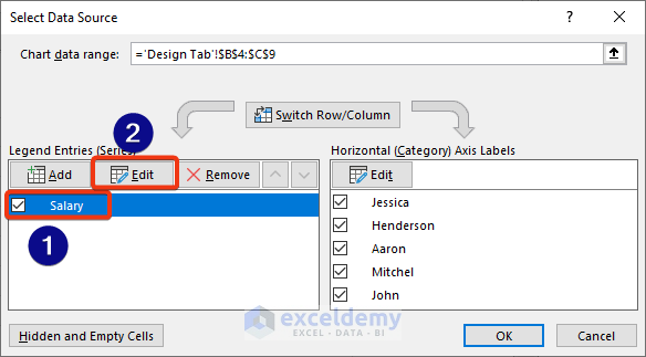
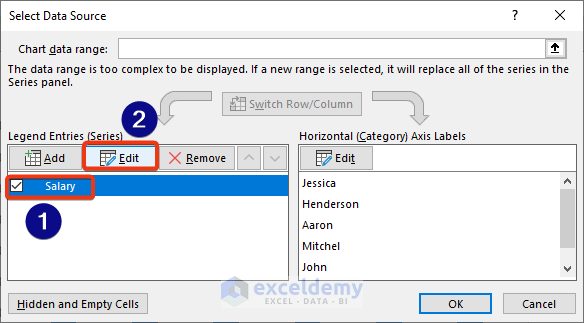
• Select Data Source window appears.
• Select the Salary option and press the Edit button.

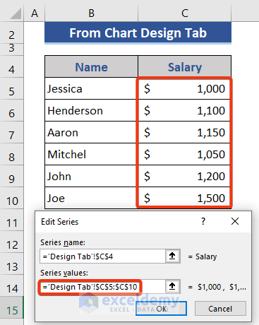
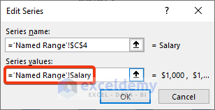
• Change the range of the Series values box and press OK.

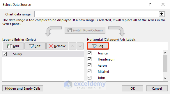
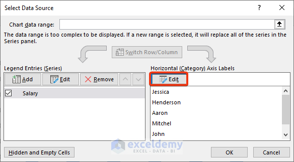
• Go to the Horizontal Axis Labels section.
• Click the Edit option.

• In the Axis label range, the box changes the range from the dataset.
• Press OK.

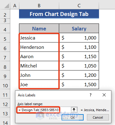
• Look at the dataset.

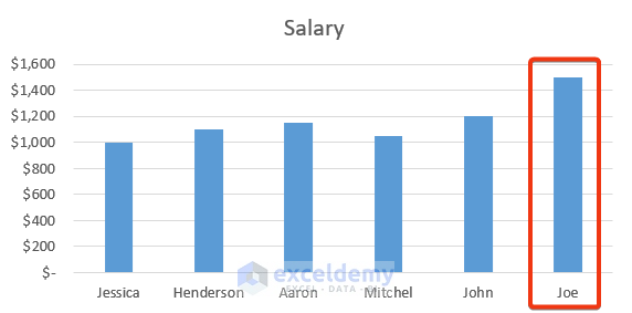The chart has been extended with the new data.

Method 2 – Expand Chart Data Range from Right-Click Context Menu

Steps:

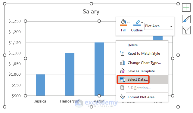
• Click the Chart first.
• Press the right button of the mouse.
• Choose Select Data from the Context Menu.

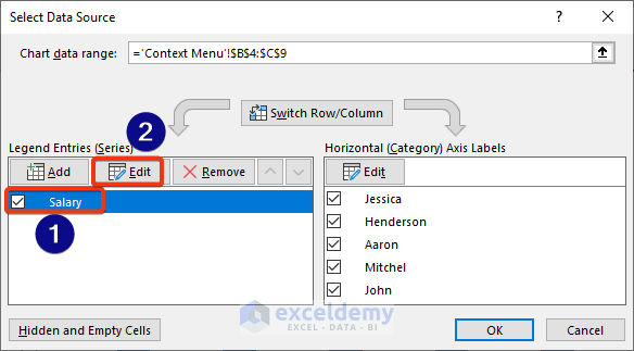
• The Select Data Source options appear now.
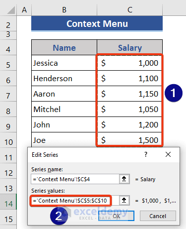
• Choose Salary and press the Edit button.

• The Edit Series window appears.
• Go to the Series values box and modify the range.
• Press OK.

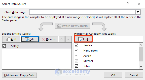
• Go back to the Select Data Source window.
• Select the Edit option of the Horizontal Axis Labels section.

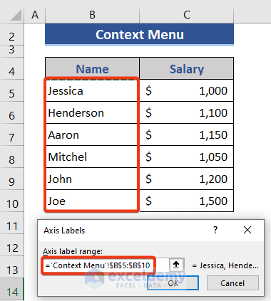
• Axis Labels window comes now.
• Modify the Axis Label range. Go to the box and select the range from the dataset.
• Press OK.

• Look at the chart.

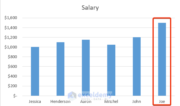
The data range of the chart has expanded successfully.

Method 3 – Use Mouse Pointer to Expand Data Range

Steps:

• Click the chart first.
• The data range is in the editable mode.
• Place the cursor on the dataset.
• Move the cursor downwards.

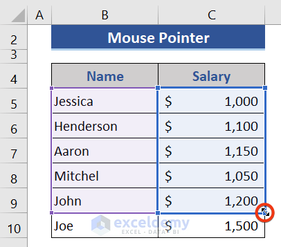
• Look at the dataset now.

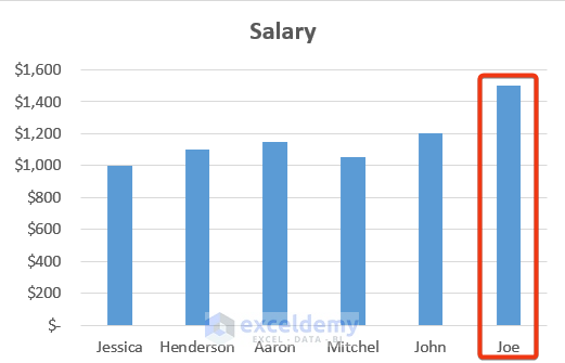The expanded data is reflected on the chart.

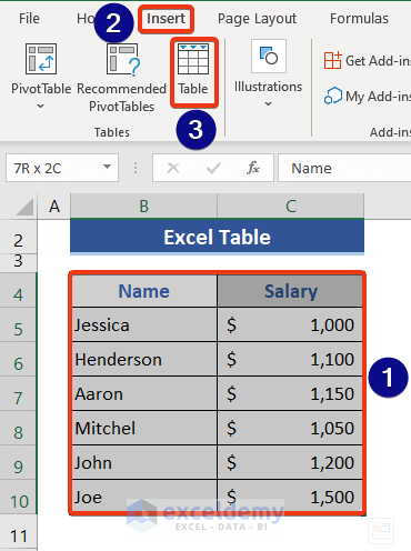
Method 4 – Utilize Excel Table Command

Steps:

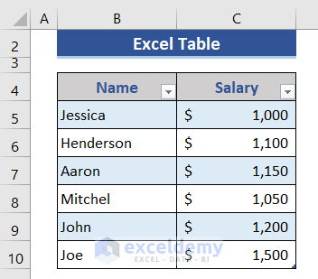
• Form an Excel Table.
• Select Range B4:C10.
• Go to the Insert tab.
• Click the Table option.

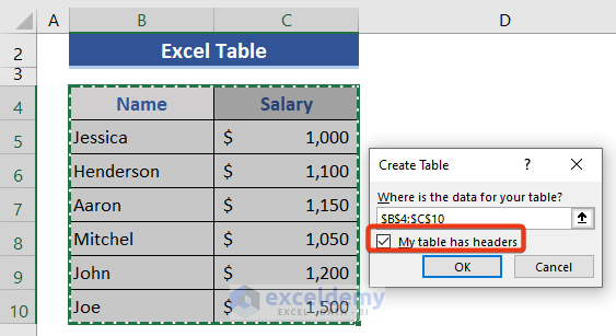
• Create Table window appears.
• Check My Table has headers option at this window.
• Press OK.

• Excel Table has formed successfully.

• Form the chart using this table.
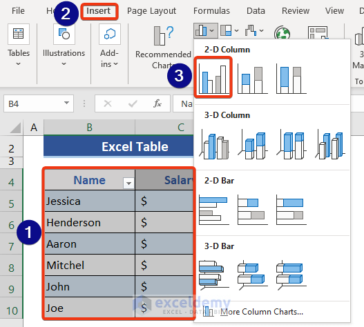
• Select the whole table.
• Go to the Insert tab.
• Choose the 2-D Column from the menu.

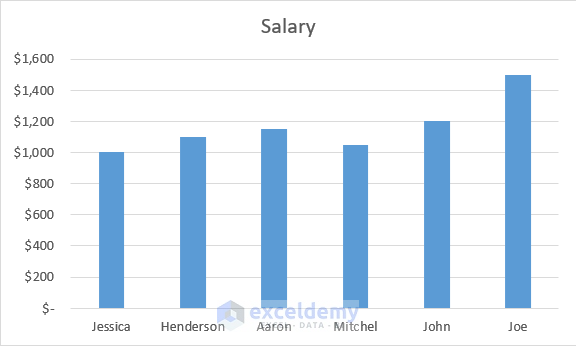
• See a chart has been created successfully.

• Expand the table.
• Copy-paste or directly write data below the last cell of the table.
• Have a look at the dataset.

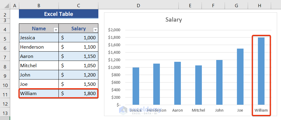We can see new data is shown in the chart.

Method 5 – Set a Dynamic Formula with Named Range to Each Data Column

Steps:

• We need to define the name range for each data column.
• Click Cell B4.
• Go to the Formulas tab.
• Choose the Define Name option.

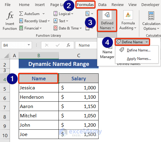
• The New Name window appears.
• Put a name in the Name box.
• Select the worksheet from the Scope dropdown.
• Insert a formula on the Refers to field.

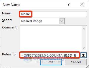
• Press OK.
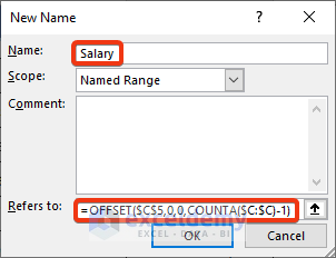
• Repeat this process for the second column.
• Named as Salary and put the formula below.

• This is our chart that has already been formed using the process shown in method 1.

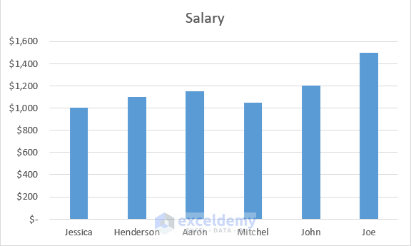
• Apply the named range here and make it dynamic.
• Click the chart.
• Press the right button of the mouse.
• Choose the Select Data option from the Context Menu.

• Select Data Source window appears.
• Select Salary and then click the Edit button.

• Edit Series window appears.
• Change the Series value reference. Put the named range reference here.

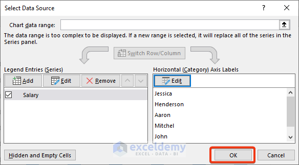
• Back to the Select Data Source window.
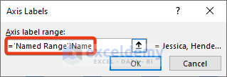
• Press the Edit option of the Horizontal Axis Labels option.

• Modify the Axis label range window.
• Press OK.

• Press OK.

• Add data to the bottom of the dataset.

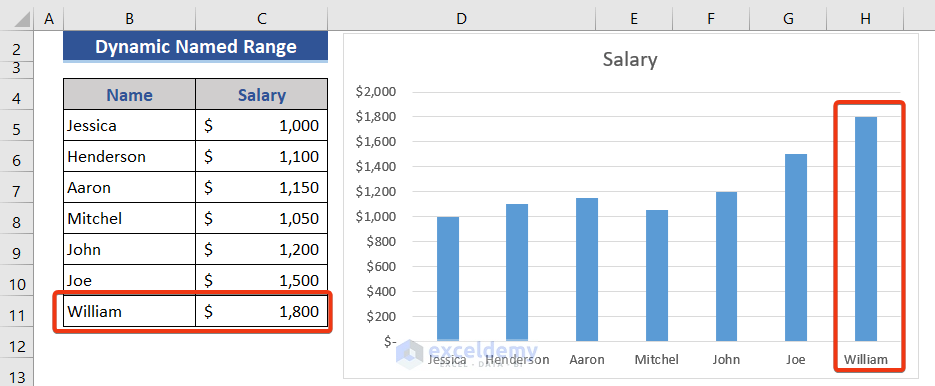
As a result, a new column appears in the chart.

Download Practice Workbook

Download this practice workbook to exercise while you are reading this article.

Related Articles

• How to Add Data Points to an Existing Graph in Excel
• How to Create Excel Chart Using Data Range Based on Cell Value
• How to Get Data Points from a Graph in Excel

<< Go Back to Edit Chart Data | Excel Chart Data | Excel Charts | Learn Excel