STEP 1 – Create Excel Column Chart
- Create a column chart.
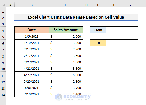
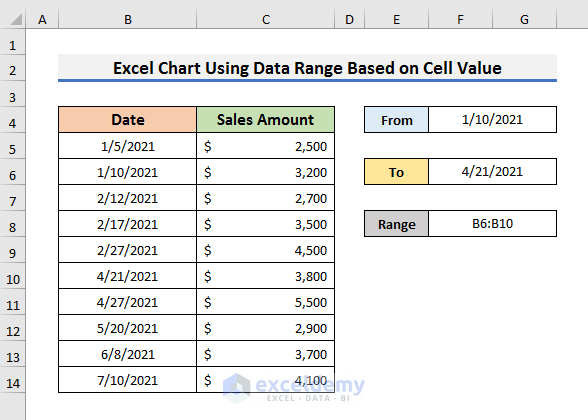
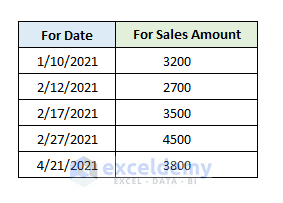
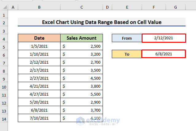
- Create a section where you will enter the dates.
- We have created From and To
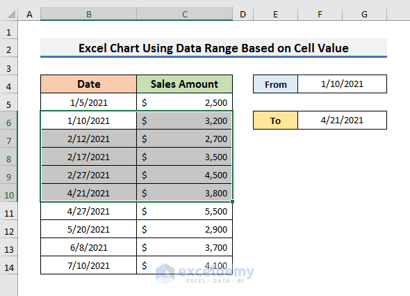
- Select the range B6:C10.
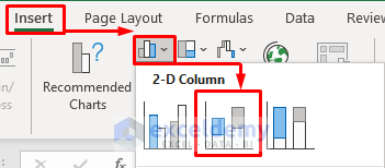
- Go to the Insert tab and select the Insert Column or Bar Chart A drop-down menu will occur.
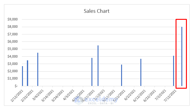
- Select Stacked Column.
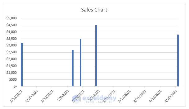
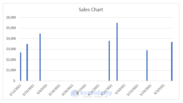
- It will output a Sales Chart.
Read More: Selecting Data in Different Columns for an Excel Chart
STEP 2 – Generate Necessary Formulas for Name Manager
- Generate formulas for the dataset below. Select the range from the date 1/10/2021 to the date 4/21/2021. It denotes the range B6:B10.
- Select any cell in the dataset and enter the formula below:
=INDEX($B$5:$B$14,MATCH($F$4,$B$5:$B$14,0)):INDEX($B$5:$B$14,MATCH($F$6,$B$5:$B$14,0))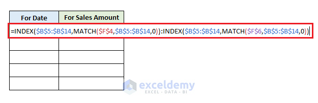
In this formula, we have used the INDEX and MATCH functions together. This formula returns the range B6:B10. Here, we have two formulas separated by the colon (:) sign.
- INDEX($B$5:$B$14,MATCH($F$4,$B$5:$B$14,0))
This is the first part of the formula that returns Cell B6. The MATCH function looks for Cell F4 in the array B5:B14 and returns the row number in that array. The output of MATCH($F$4,$B$5:$B$14,0) is 2. The formula becomes INDEX($B$5:$B$14,2) and returns the date 1/10/2021 stored in Cell B6.
- INDEX($B$5:$B$14,MATCH($F$6,$B$5:$B$14,0))
The second part of the formula returns Cell B10. The MATCH function looks for Cell F6 in the array B5:B14 and returns the row number in that array. The output of MATCH($F$6,$B$5:$B$14,0) is 6. The formula becomes INDEX($B$5:$B$14,6) and returns the date 4/21/2021 stored in Cell B10.
- Press Enter to get the results.
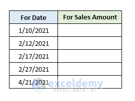
- Select another cell and enter the formula:
=INDEX($C$5:$C$14,MATCH($F$4,$B$5:$B$14,0)):INDEX($C$5:$C$14,MATCH($F$6,$B$5:$B$14,0))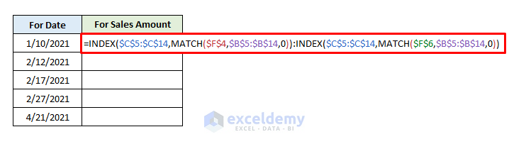
We have used the INDEX and MATCH functions together. The formula will look for the range C6:C10. It will return the desired sales amount.
- INDEX($C$5:$C$14,MATCH($F$4,$B$5:$B$14,0))
This part of the formula returns Cell C6. The MATCH function looks for Cell F4 in the array B5:B14 and returns the row number in that array. The output of MATCH($F$4,$B$5:$B$14,0) is 2. The formula becomes INDEX($C$5:$C$14,2) and returns the sales amount of $3200 stored in Cell C6.
- INDEX($C$5:$C$14,MATCH($F$6,$B$5:$B$14,0))
- Press Enter to get the results.
STEP 3 – Paste Formulas in Name Manager
- Enter the following formula below:
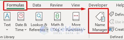
=INDEX($B$5:$B$14,MATCH($F$4,$B$5:$B$14,0)):INDEX($B$5:$B$14,MATCH($F$6,$B$5:$B$14,0))- Go to the Formulas tab and select Name Manager. It will open the Name Manager window.
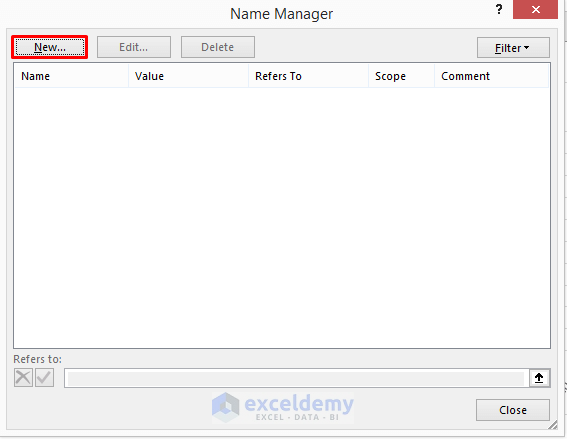
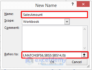
- Select New. It will open the New Name message box.
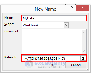
- Enter a name for the formula and paste the formula in the ‘Refers to’ field.
- We have named the formula MyDate.
- Click OK to proceed.
- Enter the formula below:
=INDEX($C$5:$C$14,MATCH($F$4,$B$5:$B$14,0)):INDEX($C$5:$C$14,MATCH($F$6,$B$5:$B$14,0))- Navigate to the Formulas tab and select Name Manager.
- Click on New.
- Enter the name in the ‘Name’ box and paste the formula in the ‘Refers to’ box.
- Click OK.
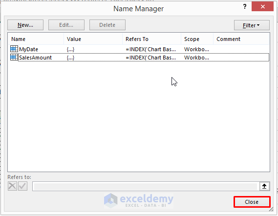
- The New Manager window will look as shown below.
- Click Close.
STEP 4 – Add Formulas in Select Data Source Window
- Add the formulas in the Select Data Source window that was created in Name Manager.
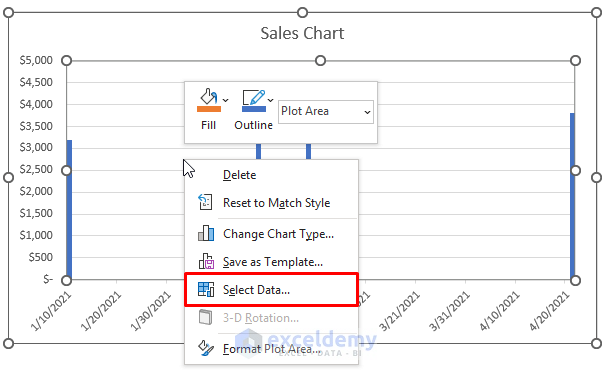
- Right–click on the chart and click on Select Data.
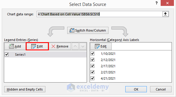
- Click on Edit in the Legend Entries section.
- Enter =‘Chart Based on Cell Value!’$C$4 in the Series name box or enter ‘=Sales Amount’.
- Enter =‘Chart Based on Cell Value!’SalesAmount in the Series values box.
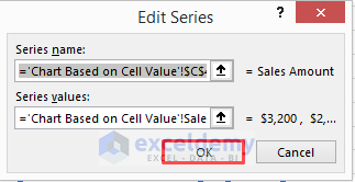
Note: In the Series values box, you need to type =‘Sheet Name!’Formula Name that is given in Name Manage. Because excel will show a warning message if you just enter the formula name.
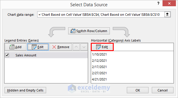
- Click on Edit in the Horizontal Axis Labels section of the Select Data Source window.
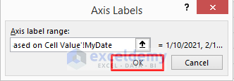
- In the Axis Labels dialog box, enter ‘Chart Based on Cell Value!’MyDate and click OK to proceed.
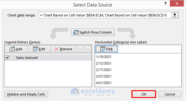
- Click OK.
Read More: How to Add Data to an Existing Chart in Excel
STEP 5 – Create Chart Using Data Range
- To know if the method works.
- Enter 2/12/2021 in Cell F4 and 6/8/2021 in Cell F6.
- You will see an update in the Sales Chart. It will show the sales amount from 2/12/2021 to 6/8/2021.
Read More: How to Expand Chart Data Range in Excel
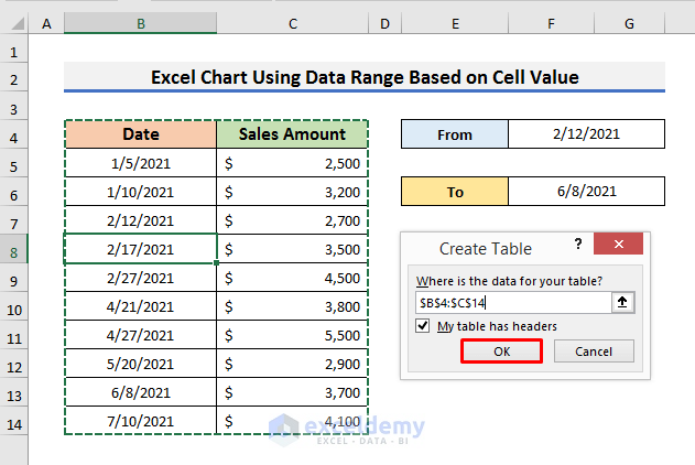
STEP 6 – Insert Excel Table to Make Dynamic Range
- We will show how you can add more sales amount information in the range and update the chart.
- Select any cell in the dataset and press Ctrl + T.
- A Create Table window will appear.
- Click OK to proceed.
- Add another date and sales amount in Cell B15 and C15.
- Enter that in Cell F6.
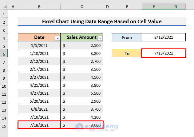
- The dataset will be updated and you will see the sales amount of 7/8/2021 on the Sales Chart.
Download Practice Book
Related Articles
- How to Add Data Table in an Excel Chart
- How to Format Data Table in Excel Chart
- How to Add Data Points to an Existing Graph in Excel
- How to Get Data Points from a Graph in Excel
<< Go Back to Data for Excel Charts | Excel Charts | Learn Excel
Get FREE Advanced Excel Exercises with Solutions!
