How to Add a Data Table to an Excel Chart – 4 Methods

Method 1 – Add a Data Table using the Chart Design Tab in Excel

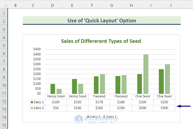
1.1. Show the Data Table Using the ‘Quick Layout’ Option

Steps:

• Click the chart and go to Chart Design > Quick Layout.
• Choose a default chart layout that includes a data table.

You will see the chart containing the data table.

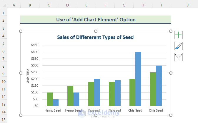
1.2. Use the ‘Add Chart Element’ Option to Show Data Tables 

Steps:

• Click any area in the chart.

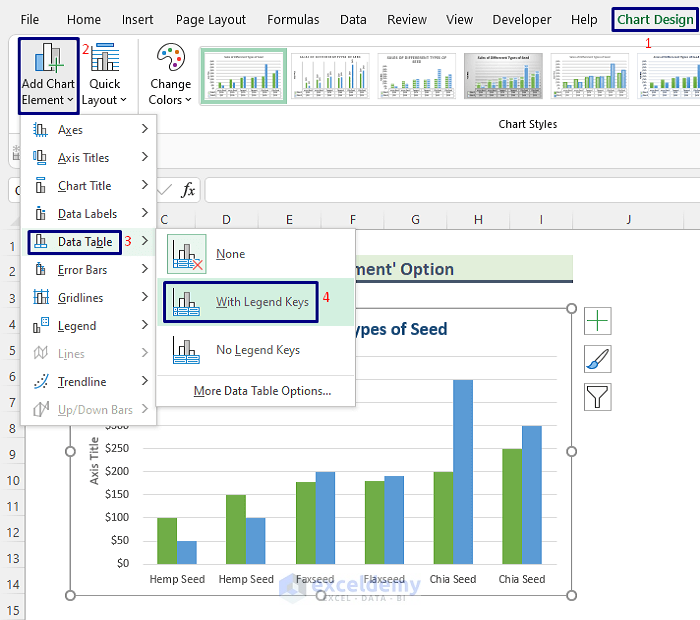
• Go to Chart Design > Add Chart Element > Data Table > With Legend Keys. You can choose No Legend Keys if you want to.

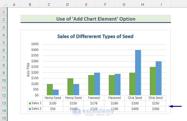
A data table is added below the chart.

Read More: How to Add Data to an Existing Chart in Excel

Method 2 – Show/Hide a Data Table by Clicking the Plus (+) Sign in an Excel Chart

Steps:

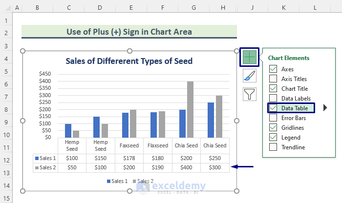
• Click any area in the chart and you will see the plus (+) sign at the top right corner.
• Click the plus sign and in Chart Elements, check Data Table.

A data table will be displayed in the chart.

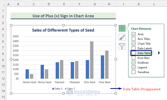
• By unchecking Data Table, you can hide the source data.

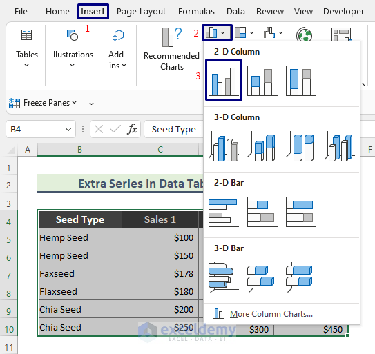
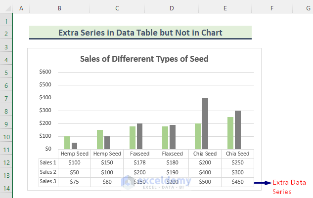
Method 3 – Add Extra Data Series to a Data Table but Not to the Chart

Steps:

• Select the source data and go to the Insert tab.
• Choose a charts option. 2-D Column, here.

This is the output.

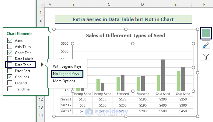
• In Chart Elements, select Data Table.
• Choose No Legend Keys.

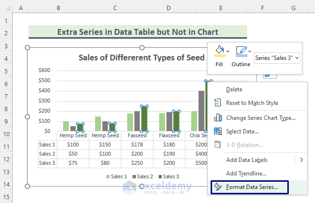
• Right-click the column you do not want to show on the chart and choose Format Data Series.

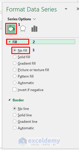
• In the Format Data Series window, select Series Options: Fill & Line.
• In Fill, click No fill.

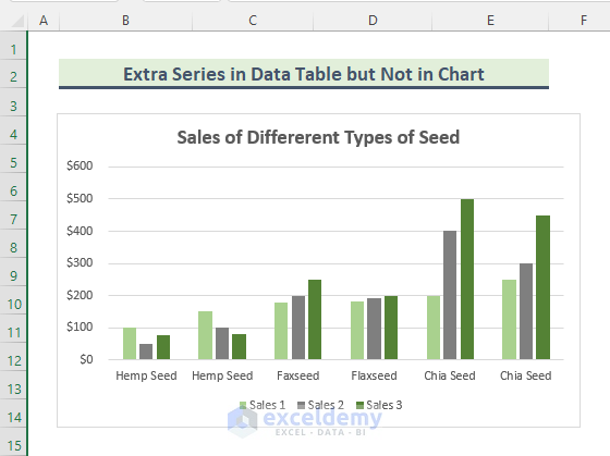
This is the output. (Extra legend key must be removed)

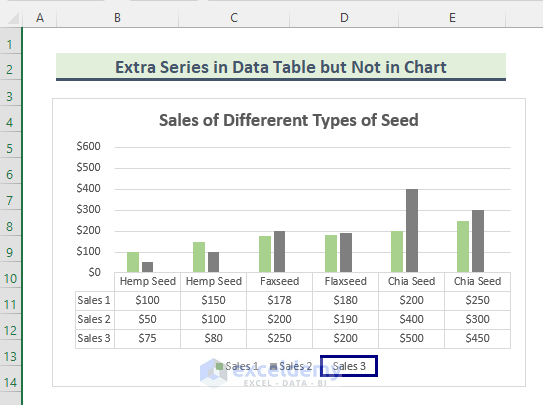
• Go to Chart Design > Add Chart Element > Legend > None.

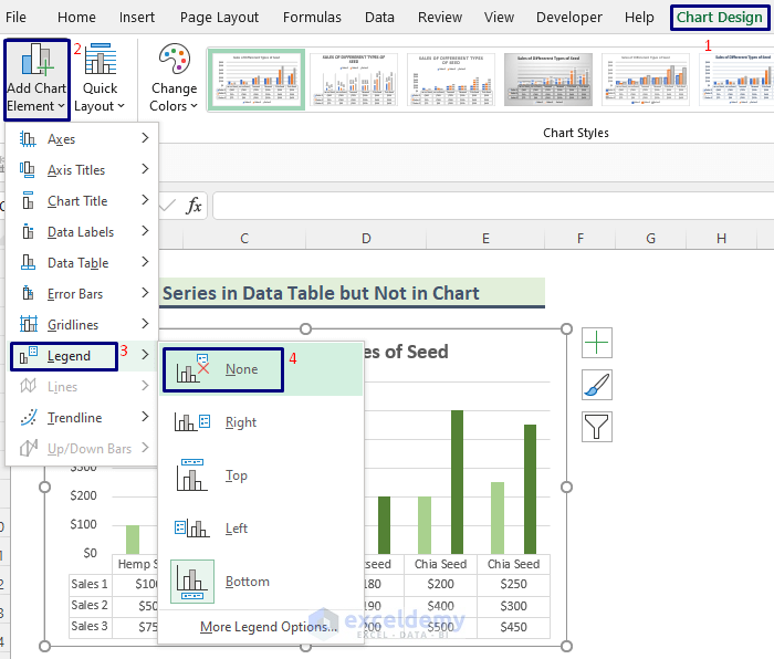
This is the final output.

Method 4 – Format a Data Table in an Excel Chart

Steps:

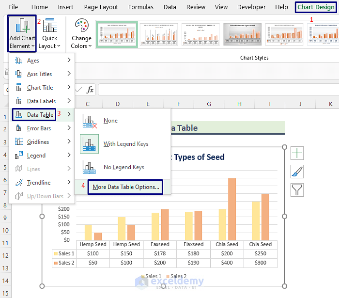
• Click the chart and go to Chart Design > Add Chart Element > Data Table > More Data Table Options.

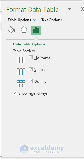
• In the Format Data Table window, selected your format.

Download Practice Workbook

Download the practice workbook here.

Further Readings

• How to Select Data for a Chart in Excel
• Selecting Data in Different Columns for an Excel Chart
• How to Expand Chart Data Range in Excel
• How to Add Data Points to an Existing Graph in Excel
• How to Create Excel Chart Using Data Range Based on Cell Value
• How to Get Data Points from a Graph in Excel

<< Go Back to Data for Excel Charts | Excel Charts | Learn Excel