How to Sort Data in Excel Chart (5 Easy Methods)

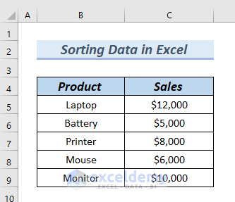
In the following dataset, you can see the Product and Sales columns. Using this dataset, we will insert a Bar chart.

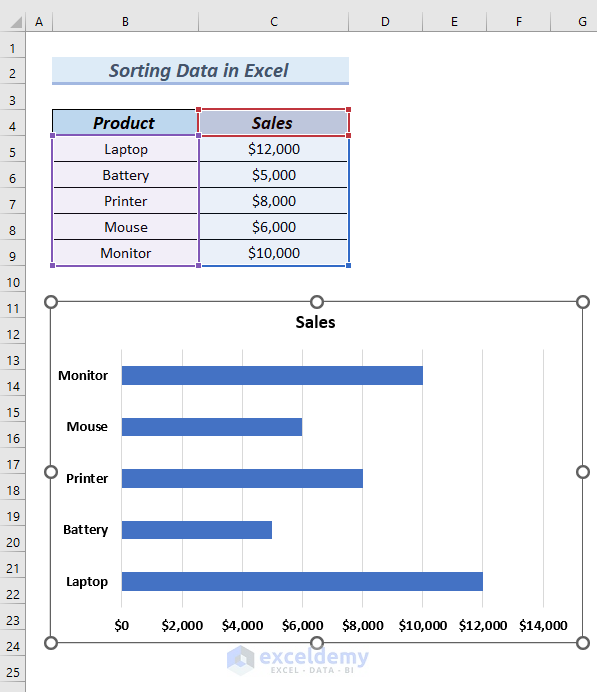
• Select the entire dataset and go to the Insert tab.
• From the Insert Column or Bar Chart group, select a 2D Clustered Bar chart.

We will use the bar chart to show how you can sort data.

Method 1 – Using the Sort Feature to Sort Data in an Excel Chart

Steps:

• Insert a Bar chart by following the steps described earlier.
• Select cells B4:C9 and go to the Data tab.
• From the Sort & Filter group, select the Sort option.

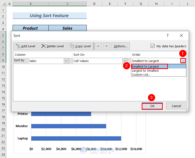
• A Sort dialog box will appear.
• Click on the downward arrow of the Order box and select Smallest to Largest.
• Click OK.

• You can see the dataset has been sorted and the Bar chart along with it.

Read More: How to Edit Chart Data in Excel

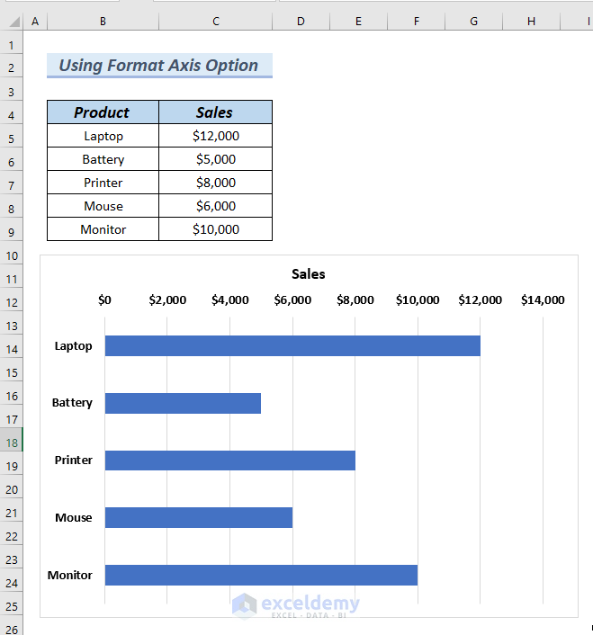
Method 2 – Using the Format Axis Feature in Excel

Steps:

• Insert a Bar chart by following the steps described earlier.

• Select the Y axis of the Bar chart and right-click on it.
• Select Format Axis from the Context Menu.

• A Format Axis dialog box will appear on the right side of the Excel sheet.
• Mark the Categories in reverse order box.

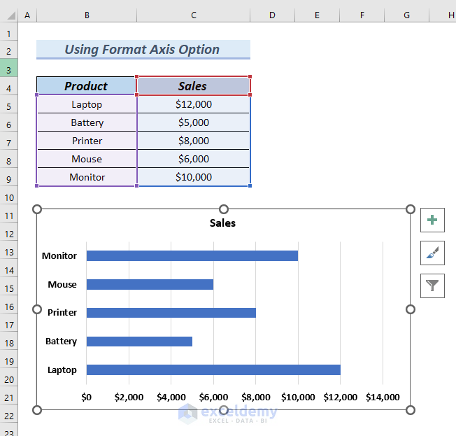
• You can see the sorted chart in Excel. The data table of the chart remains the same.

Read More: How to Change X-Axis Values in Excel

Method 3 – Sorting the Data Table to Sort Chart Data

Steps:

• Select the dataset from cells B4:C9 and go to the Insert tab.
• From the Tables group, select Table.

• A Create Table dialog box will appear.
• Make sure My table has headers is marked and click OK.

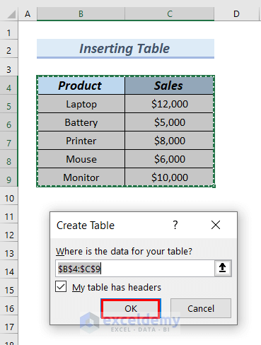
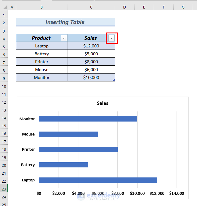
• Excel converts the data into a Table.

• Insert a Bar chart using the steps described earlier.
• Click on the drop-down arrow of the Sales column.

• Select the Sort Largest to Smallest option.
• This will sort the Table and the chart from largest to smallest.

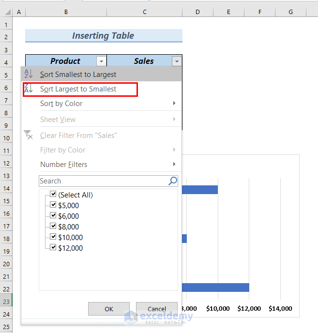
• You can see the sorted data in an Excel chart on the screenshots.

Method 4 – Utilizing the SHIFT Key and Mouse to Sort Data

Steps:

• Insert a Bar chart using the steps described earlier.

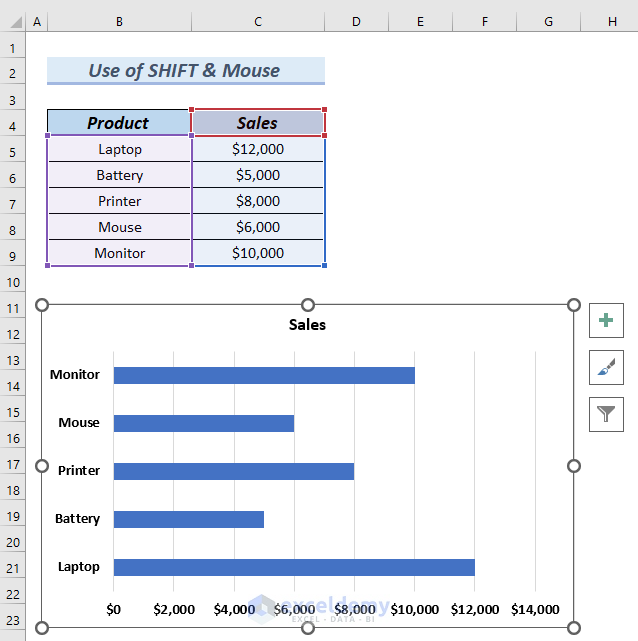
• Select cells B5 and C5 and hold the Shift key.

• A four-directional arrow will pop up.
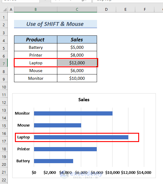
• While holding the SHIFT key, click and drag the cells to the desired place.

• We moved the cells to B7 and C7.
• Release the Mouse and Shift.

Method 5 – Inserting a Pivot Table to Sort Data in an Excel Chart

Steps:

• Select cells B4:C9.
• From the Insert tab, select the PivotChart group.
• Select Pivot Chart.

• A Create PivotChart dialog box will appear.
• Select New Worksheet and click OK.

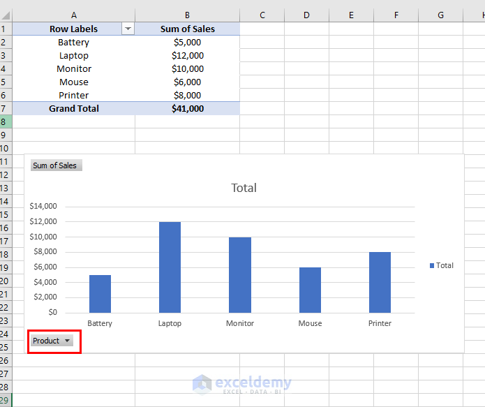
• A PivotTable Fields dialog will appear in a new Worksheet.
• Drag Product into the Rows group.
• Drag Sales into the Values group.

• Click on Product of the Column chart.

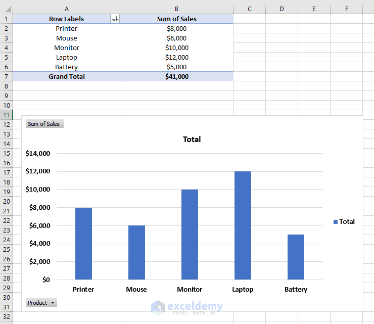
• Select Sort Z to A.
• This will sort the chart data from Z to A in alphabetical order.

• Both charts have also been sorted alphabetically from Z to A.

Practice Section

You can download the sample Excel file to practice.

Download Practice Workbook

Related Articles

• How to Change Chart Data Range in Excel
• How to Edit Data Table in Excel Chart
• How to Change Data Source in Excel Chart
• How to Change Chart Data Range Automatically in Excel
• How to Group Data in Excel Chart
• How to Limit Data Range in Excel Chart
• How to Skip Data Points in an Excel Graph
• How to Remove One Data Point from Excel Chart
• How to Hide Chart Data in Excel

<< Go Back to Data for Excel Charts | Excel Charts | Learn Excel