Stem and leaf plots are useful tools for organizing and displaying numerical data. They provide a simple way to visually represent data without losing information, making them popular in fields such as statistics, finance, and engineering. While there are many software programs that can create stem and leaf plots, Microsoft Excel is a popular choice due to its widespread availability and ease of use. In this article, we will provide step-by-step instructions on how to make a stem and leaf plot in Excel. Whether you’re a student, researcher, or data analyst, this guide will help you create informative and visually appealing stem and leaf plots using Excel.
Introduction to Stem and Leaf Plot
What Is Stem and Leaf Plot?
A stem and leaf plot is a graphical representation of a set of numerical data that displays each data point by splitting it into a stem (the leading digits) and a leaf (the trailing digits). The stem and leaf plot allows us to organize and visualize data in a way that shows the distribution and frequency of the data points. In Excel, a stem and leaf plot can be created using the REPT, LEFT, and RIGHT functions in combination with various Excel options. The resulting plot can help us identify patterns, outliers, and other features of the data set that may not be apparent from a simple list of numbers. Overall, stem and leaf plots are useful tools for exploring and communicating numerical data in a clear and concise manner.
Benefits of Using Stem and Leaf Plot
The advantages of using a stem and leaf plot are that it shows the distribution of the data and keeps the actual values, which can be useful for small datasets or when you need to look at individual values. It is also easy to create and understand, even for people without knowledge of statistical analysis.
Limitations of Using Stem and Plot
There are some limitations to using a stem and leaf plot. It can be time-consuming to create it for large datasets, and it may not be as effective for visualizing all types of data, such as skewed distributions or outliers. Additionally, it may not be as known or intuitive to some people as other types of graphs or charts.
How to Make Stem and Leaf Plot in Excel: 3 Simple Methods
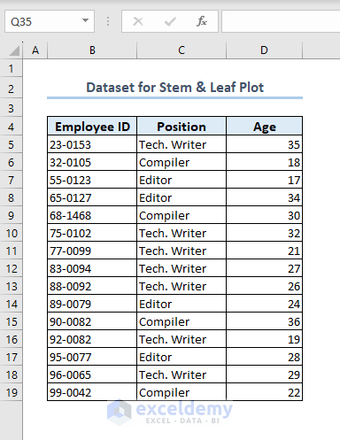
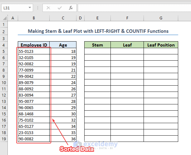
In this segment, we will discuss 3 simple methods to make a stem and leaf plot in Excel. Without any further delay, let’s jump to the procedures. For demonstration, we have used a dataset with Employee ID, Position and Age. We will make a stem and leaf plot with the Age column’s data, as it contains 2 digits.
1. Making Stem & Leaf Plot with REPT & COUNIF Functions
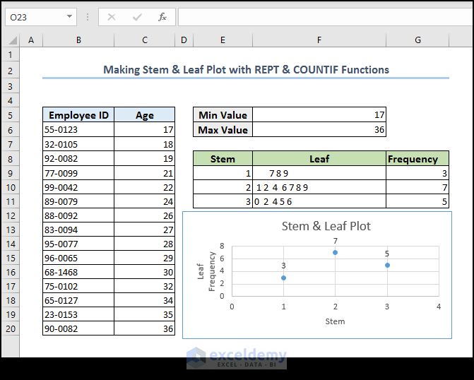
In the first method, we will use the REPT and COUNTIF functions to calculate stem, leaf, and frequency for plotting.
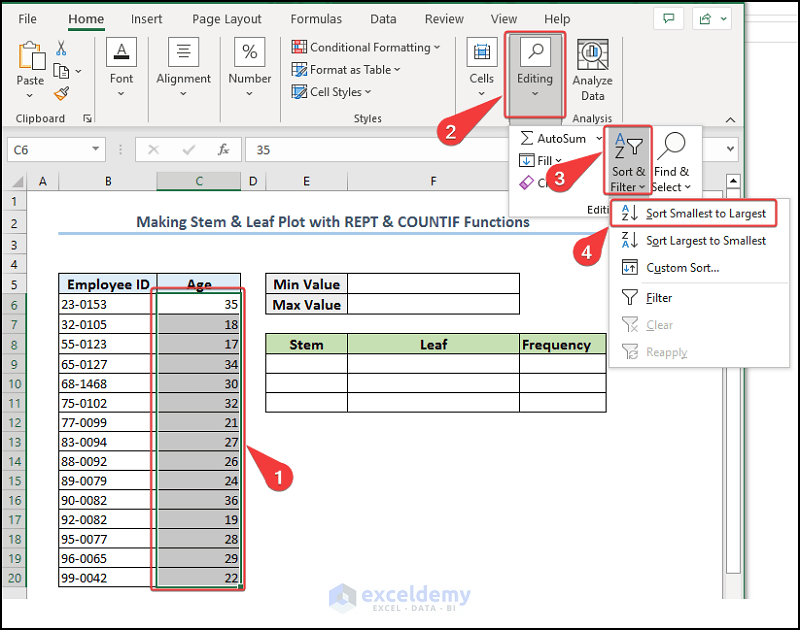
- Firstly, select the data from the Age column and select Home tab > Editing > Sort & Filter > Sort Small to Largest to sort them in ascending order. You can scape this step, but sorting the data helps to visualize them easily.
- Afterward, use the MIN & MAX functions to determine the maximum and minimum values of the data from the Age column. You can use the below formula for F5 cell.
=MIN(C5:C19)And the formula for F6 cell is-
=MAX(C5:C19)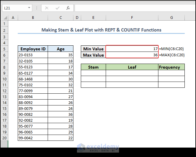
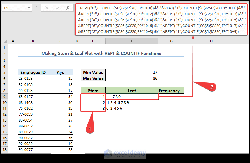
- Next, enter the stems which are the first digits of our data. For example, stem for E9 cell will be 1 for 17, 18, 19 ages.
- Then, for determining the leaf, you can use the following formula.
=REPT("0",COUNTIF($C$5:$C$19,E8*10+0))&" "&REPT("1",COUNTIF($C$5:$C$19,E8*10+1))&" "&REPT("2",COUNTIF($C$5:$C$19,E8*10+2))&" "&REPT("3",COUNTIF($C$5:$C$19,E8*10+3))&" "&REPT("4",COUNTIF($C$5:$C$19,E8*10+4))&" "&REPT("5",COUNTIF($C$5:$C$19,E8*10+5))&" "&REPT("6",COUNTIF($C$5:$C$19,E8*10+6))&" "&REPT("7",COUNTIF($C$5:$C$19,E8*10+7))&" "&REPT("8",COUNTIF($C$5:$C$19,E8*10+8))&" "&REPT("9",COUNTIF($C$5:$C$19,E8*10+9))
Formula Breakdown:
- REPT(“0”,COUNTIF($C$5:$C$19,E8*10+0)): This uses the REPT function to repeat the character “0” a number of times equal to the count of values in the range $C$5:$C$19 that have a decimal part between E8*10+0 and E8*10+0.9. Here, E8 is the stem value. For example, if the stem value is 3, then E8*10+0 would be 30, and this part of the formula would count the number of values in the range that have a decimal part between 30 and 30.9, and repeat the character “0” that many times.
- &” “&REPT(“1″,COUNTIF($C$5:$C$19,E8*10+1))&” “: This concatenates a space character with the REPT function that repeats the character “1” a number of times equal to the count of values in the range that have a decimal part between E8*10+1 and E8*10+1.9. This is repeated for each digit from 0 to 9, with a space character separating each group of asterisks.
- The end result is a string of asterisks that represents the frequency of each decimal value within the stem.
- Next, use the Fill Handle of Excel to copy the formula and determine other leaves.
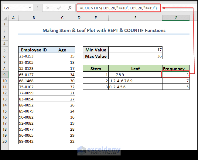
- Afterward, use the following formula in cell G9 to count the leaf number for a stem. Also, for other counts, use similar formulas.
=COUNTIFS(C5:C19,">=10",C5:C19,"<=19")In the formula, COUNTIFS is a function that counts the number of cells that meet one or more criteria.
- C5:C19: This is the range of cells being evaluated.
- “>=10“: This is the first criterion. It checks if the value in each cell is greater than or equal to 10.
- C5:C19,”<=19“: This is the second criterion. It checks if the value in each cell is less than or equal to 19.
- The two criteria are combined using the COUNTIFS function. The function counts the number of cells that meet both criteria, i.e., has a value between 10 and 19.
So the formula counts the number of cells in the range C5:C19 that have a value between 10 and 19 (inclusive).
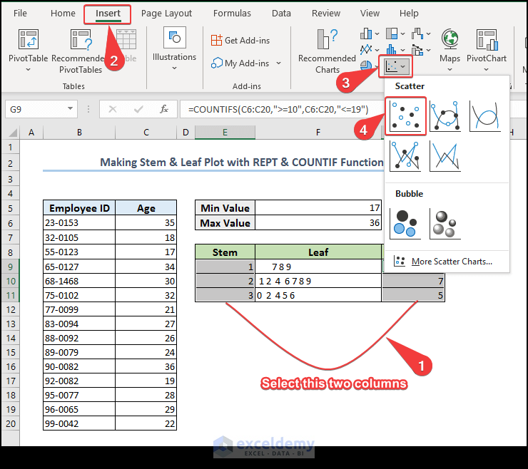
- Further, select the Stem & Frequency column data and select Insert > Chart > Scatter.
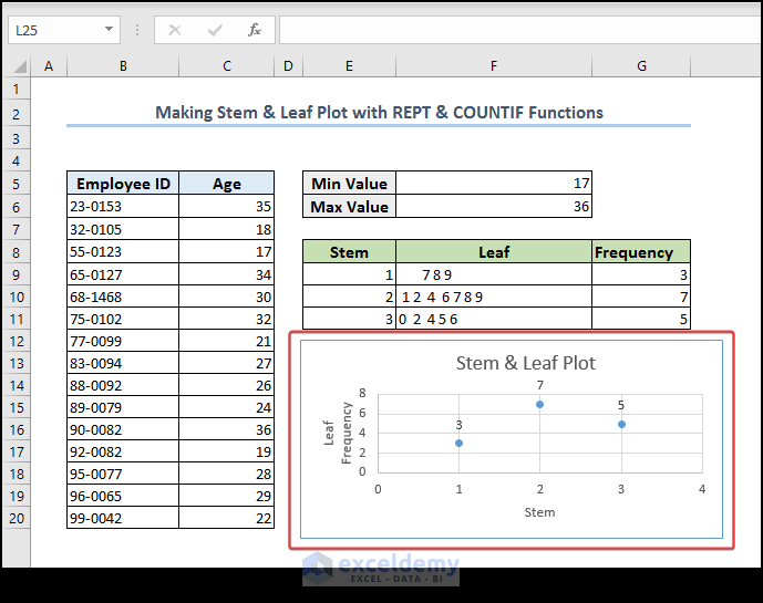
- Finally, do some formatting to the plotting and get a result plotting like the one included in the following image. This is our stem & leaf plot.
Read More: Back to Back Stem and Leaf Plot Excel
2. Creating Stem & Leaf Plot Using LEFT-RIGHT & COUNTIF Functions
This time, we will do the same task in Excel but in a bit of a different manner. We will show the stem number separately for each leaf with the help of the LEFT and RIGHT functions. Let’s see the procedures.
- Primarily, sort the data as we did in the previous method.
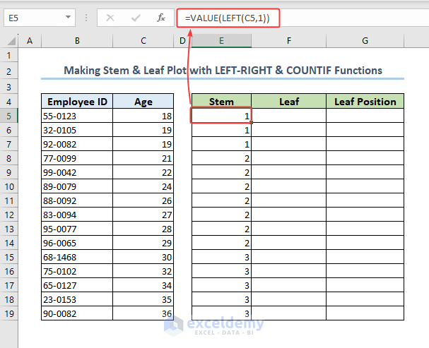
- Then, use the following formula to find the stem, which is the first digit from the numbers of the Age column. Use the Fill Handle to copy the formula to other cells to get all stem values.
=VALUE(LEFT(C5,1))In the formula, the LEFT function takes the first digit (from left) of the value from cell C5. The VALUE function converts it to a numeric value. This way, we get our stem for the plot.
- Further, apply the following formula for determining the leaf values. Also, use the Fill Handle again.
=VALUE(RIGHT(C5,1))In the formula, the RIGHT function takes the first digit (from the right) of the value from cell C5. The VALUE function converts it to a numeric value. This way, we get our leaf for the plot.

- Now, let’s find the leaf position of each leaf on a stem. You can use the following formula for that.
=COUNTIF($E$5:E5,E5)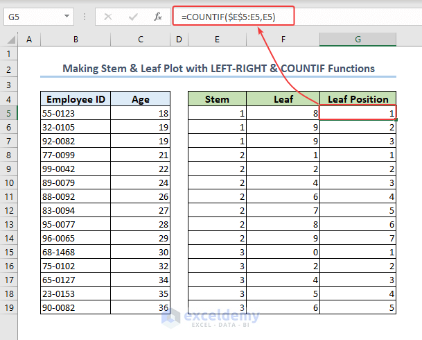
Formula Breakdown:
- COUNTIF: This is the function that counts the number of cells in a range that meet a certain criterion.
- $E$5:E5: This is the range of cells that the function will count. The first part of the range ($E$5) is an absolute reference, which means that it will always refer to cell E5, no matter where the formula is copied. The second part of the range (E5) is a relative reference, which means that it will adjust based on the position of the formula when it is copied. In this case, the range will expand as the formula is copied down the column.
- E5: This is the criterion that the function will use to count the cells. In this case, it’s the value in cell E5 itself.
- $E$5:E5: This is the dynamic range that the function will count. The dollar signs in $E$5 make this an absolute reference, which means that it will always refer to cell E5. However, the second part of the range (E5) is a relative reference, which means that it will adjust based on the position of the formula when it is copied. In this case, the range will expand as the formula is copied down the column so that it always includes all the cells above the current cell up to and including cell E5.
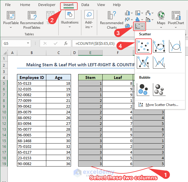
- Afterward, select data from columns Stem & Leaf Position and select Insert > Charts > Insert Scatter > Scatter for creating a scatter plot with the data.
- Finally, do some formatting on plotting and eventually, we will get a stem & leaf plot like in below image.

3. Create Stem and Leaf Plot with Decimals in Excel
Stem and leaf plots can be done with decimal numbers as well. Suppose we have numbers like 12.1, 12.5, 12.7, then 12 will be the stem and 1, 5, and 7 will be the leaves. Let’s do it in Excel.
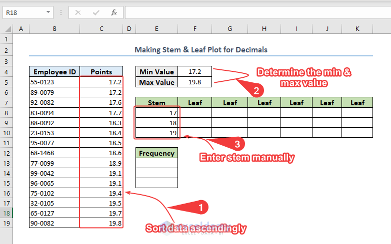
- Primarily, sort the data ascendingly as before.
- Then, find the minimum and maximum value from the data for better understanding and for further steps.
- Later on, input the stem values in the worksheet manually. Our stems are 17, 18, and 19.
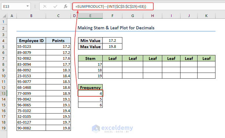
- Further, calculate the frequency of the leaf for a stem using the following formula.
=SUMPRODUCT(--(INT($C$5:$C$19)=E8))Formula Breakdown:
- SUMPRODUCT: This is a function that multiplies corresponding values in arrays and then adds the results together.
- –(INT($C$5:$C$19)=E8): This is an array that uses a combination of functions to return an array of boolean values (TRUE or FALSE). Here’s how it works:
-
- INT($C$5:$C$19) rounds down each value in the range C5:C19 to the nearest integer. This is used to separate the stem and leaf parts of each value.
-
- =(INT($C$5:$C$19)=E8) compares each integer value in the range to the stem value in cell E8. This returns an array of boolean values (TRUE if the integer matches the stem, FALSE if it doesn’t).
-
- — converts the boolean values to 1‘s (TRUE) and 0‘s (FALSE), which allows the array to be used in the SUMPRODUCT function.
- SUMPRODUCT(–(INT($C$5:$C$19)=E8)): This calculates the sum of the array of 1‘s and 0‘s. Since each 1 represents a value in the range that matches the stem value in cell E8, the sum is equal to the frequency of values that have that stem.
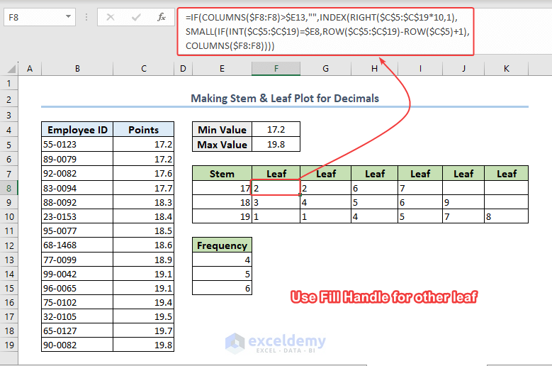
- Finally, use the following formula for determining the leaf of the decimal numbers.
=IF(COLUMNS($F8:F8)>$E13,"",INDEX(RIGHT($C$5:$C$19*10,1),SMALL(IF(INT($C$5:$C$19)=$E8,ROW($C$5:$C$19)-ROW($C$5)+1),COLUMNS($F8:F8))))Formula Breakdown:
- IF: This is a logical function that tests a condition and returns one value if the condition is true, and another value if the condition is false.
- COLUMNS($F8:F8): This returns the number of columns in the range $F8:F8. When this formula is copied across the row, the range reference will adjust to include more columns, allowing the formula to retrieve more leaf values.
- > $E13: This tests whether the number of columns is greater than the maximum number of leaves per stem. If this condition is true, the formula returns an empty string (“”), which prevents additional leaf values from being displayed.
- INDEX: This is a function that returns a value from an array based on a specified row and column number.
- RIGHT($C$5:$C$19*10,1): This returns the rightmost digit of each value in the range C5:C19 multiplied by 10. This is used to extract the leaf value for each number.
- SMALL: This is a function that returns the nth smallest value from a range or array.
- IF(INT($C$5:$C$19)=$E8,ROW($C$5:$C$19)-ROW($C$5)+1): This creates an array that contains the relative row numbers of values in the range C5:C19 that have a stem value equal to the value in cell E8. This is used to determine the row number of the leaf value that should be displayed. This part gives an array of numbers 1, 2, 3, 4.
- ROW($C$5:$C$19)-ROW($C$5)+1: This returns the relative row numbers of the values in the range C5:C19. This is used in the IF function to create an array of relative row numbers for values that have the same stem as the current stem being plotted.
- COLUMNS($F8:F8): This returns the number of columns in the range F8:F8. This is used as the second argument in the SMALL function to return the nth smallest value from the array created by the IF function.
- IF(COLUMNS($F8:F8)>$E13,””,INDEX(RIGHT($C$5:$C$19*10,1),SMALL(IF(INT($C$5:$C$19)=$E8,ROW($C$5:$C$19)-ROW($C$5)+1),COLUMNS($F8:F8)))): This is the full formula. It tests whether the number of columns is greater than the maximum number of leaves per stem. If it is, the formula returns an empty string. If not, it uses the INDEX and SMALL functions to return the leaf value for the corresponding row number.
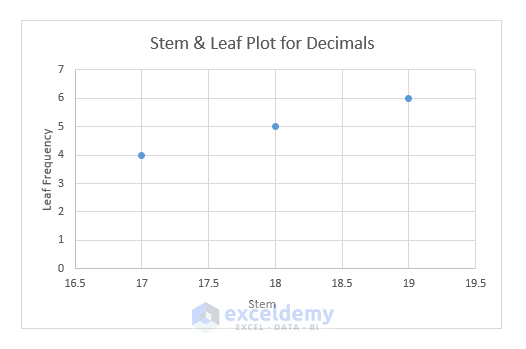
- Lastly, you can plot the step and leaf plot using the data of Stem & Frequency (leaf).
Frequently Asked Questions
1. Can we customize the appearance of our stem-and-leaf plot in Excel?
Ans: Yes, you can customize the appearance of your stem-and-leaf plot in Excel by using various formatting options, such as changing the font size and color, adding gridlines or borders, and adjusting the axis labels. You can also add a chart title or legend to make the plot more informative.
2. How to interpret a stem and leaf plot?
Ans: To interpret a stem and leaf plot, look at the distribution of the data. The stem represents the larger values (first digit from left), while the leaves represent the smaller values (second values from left). You can see how many data points fall into each group by counting the number of leaves for each stem. You can also see the range of the data by looking at the first and last stems.
3. What type of data is best suited for a stem and leaf plot?
Ans: A stem and leaf plot is best suited for numerical data with a relatively small range of values, such as test scores, temperatures, or times. It is not as useful for large datasets or continuous data.
4. What is the difference between a stem and leaf plot and a histogram?
Ans: A stem and leaf plot shows the actual values of the data, while a histogram groups the data into intervals or bins and shows the frequency of values in each bin. Histograms are better suited for larger datasets and continuous data, while stem and leaf plots are better suited for smaller datasets and discrete data.
Things to Remember
- In a few formulas, we have used specific cell ranges and in some cases, we used normal cell reference which can be changed accordingly while copying. Observe and apply the references in the formula carefully.
- In a few methods, sorting the data is required first as mandatory. but sometimes, it’s optional.
Download Practice Workbook
You can download the practice workbook from here.
Conclusion
In conclusion, creating a stem-and-leaf plot in Excel can be a useful way to visualize and analyze data, especially when dealing with small datasets. By following the steps and using the formulas provided in this article, you can create an effective stem-and-leaf plot for both whole numbers and decimal values. By applying some best practices and customizing the appearance of your plot, you can make it even more informative. Don’t hesitate to comment if you have any queries or suggestions.
Related Articles
- How to Make a Cumulative Distribution Graph in Excel
- How to Make a t-Distribution Graph in Excel
- How to Make Cumulative Percentage Polygon in Excel
- How to Create a Percentage Polygon in Excel
- How to Create Grade Distribution Chart in Excel
- How to Create Gaussian Distribution Chart in Excel
<< Go Back to Excel Distribution Chart | Excel Charts | Learn Excel
Get FREE Advanced Excel Exercises with Solutions!
