How to Create Gaussian Distribution Chart in Excel

Microsoft Office 365 was used to create this article, however you can use other versions according to your preference. If any of the steps don’t work in your version, please let us know in the comments below.

What is Gaussian Distribution Chart?

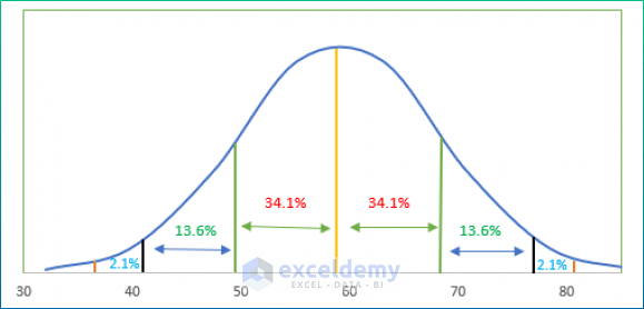
Usually, a Gaussian Distribution Chart is a graph that represents the normal distribution of a variable, otherwise known as the Normal Distribution Curve or Bell Curve. This distribution can be observed everywhere, for instance if we survey marks from an exam, most of the numbers will be in the middle. The peak point of this curve signifies the mean of the distribution, which is lower on either side. This denotes the probability, which is much lower for the extreme values (i.e. highest or lowest).

The features of the Gaussian Distribution Chart below are:

1 standard deviation of a mean is where 68.2% of the distribution falls.
95.5% of the distribution lies within the range of the average‘s two standard deviations.
99.7% of the distribution is contained within a range of three standard deviations from the mean.

excel gaussian distribution chart

How to Create a Gaussian Distribution Chart in Excel

To create a Gaussian distribution chart, we’ll use the AVERAGE, STDEV.P, and NORM.DIST functions. In general, the AVERAGE function returns the average of the numbers it takes as arguments. The STDEV.P function also takes a series of numbers as arguments and returns the standard deviations. The NORM.DIST function takes a value from a range of data, the mean and standard deviation for the dataset, and a boolean value as its arguments, and returns the normal distribution of the numbers in the range.

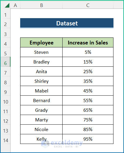
Step 1 – Select Dataset

For the purpose of demonstration, we’ll use the following sample dataset containing information about the Increase in Sales of each Employee in two consecutive months. We’ll make a Gaussian distribution chart for this increase in sales.

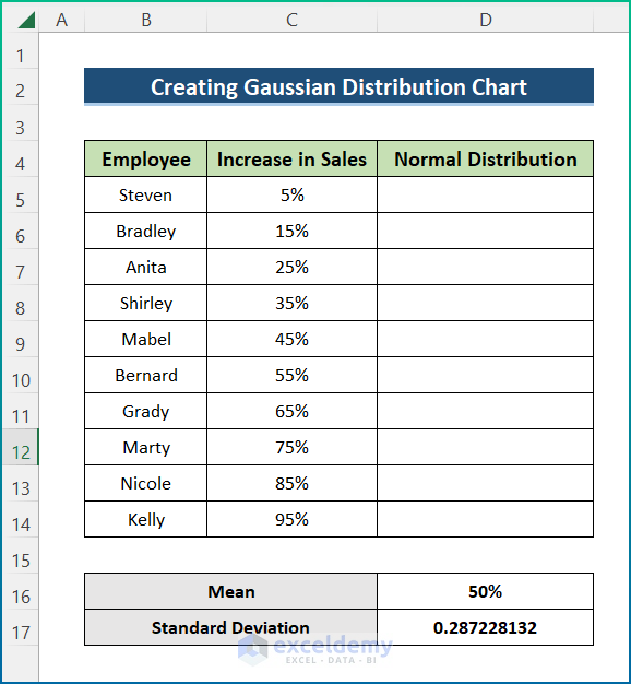
Step 2 – Calculate Mean and Standard Deviation

In cell D16 enter the following formula to find the Mean increase in sales:

=AVERAGE(C5:C14)

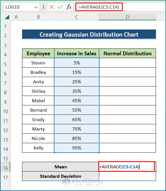
Press Enter.

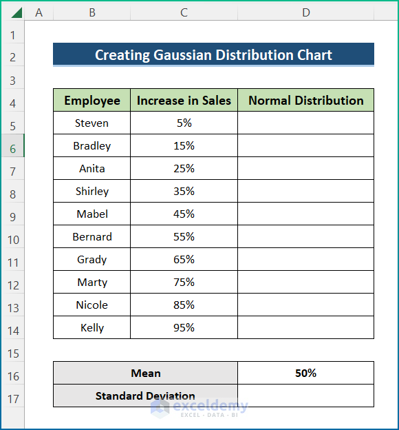
Similarly, in cell D17 enter the formula below to calculate the standard deviation:

=STDEV.P(C5:C14)

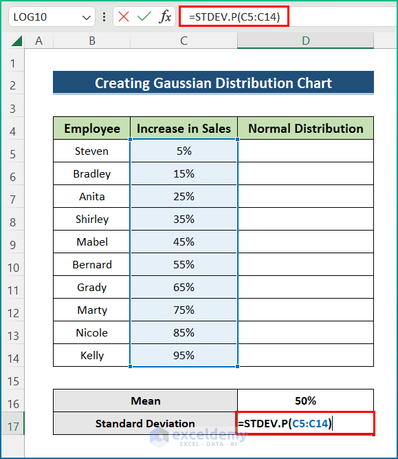
Press Enter.

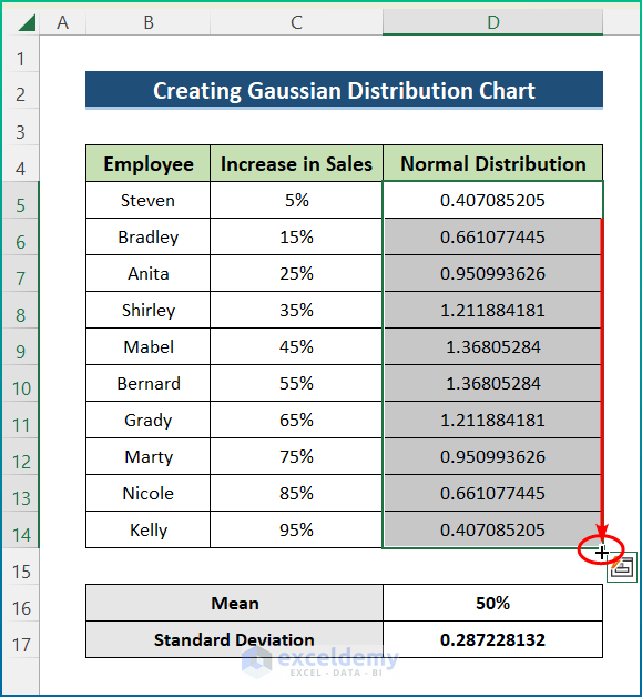
Step 3 – Determine Normal Distribution

In cell D5, enter the following formula:

=NORM.DIST(C5,$D$16,$D$17,FALSE)

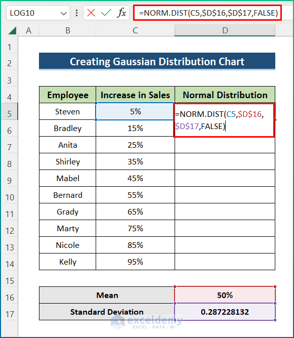
Press Enter and use the AutoFill tool to apply the formula to the entire column.

Step 4 – Create Gaussian Distribution Chart

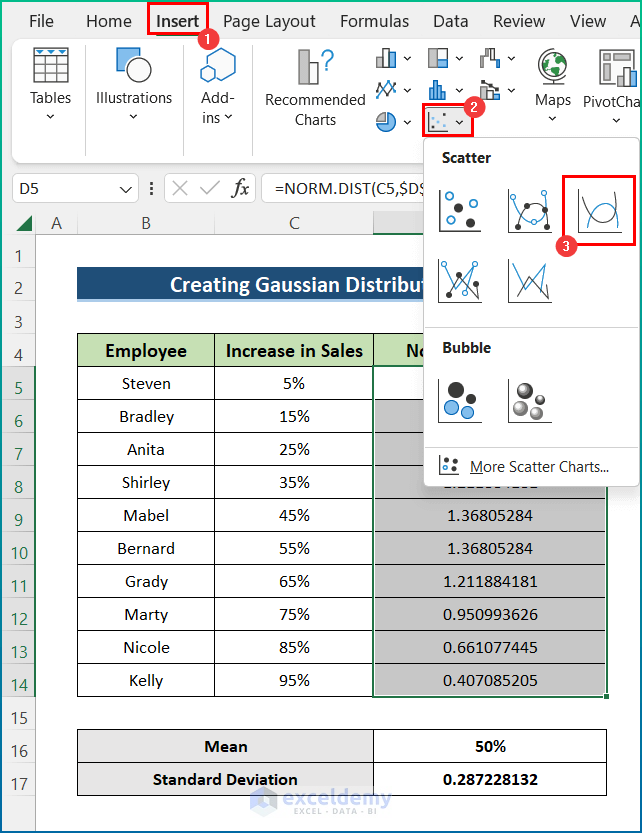
Select the range D5:D14.
Click the Insert tab.
Click on the Scatter command from the Charts group.
Choose Scatter with Smooth Lines.

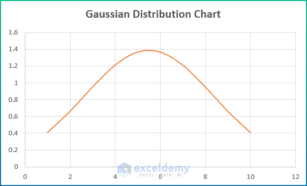
Final Output

The following Gaussian Distribution Chart is returned. After some formatting modifications, the chart looks as follows:.

Things to Remember

It is recommended to sort the data before plotting the normal distribution, otherwise an irregular curve may occur.
Then select the chart to access the Chart Element menu and other chart editing options, and modify the chart according to your personal preference.
The mean and standard deviation of the data must be numeric, else a #VALUE error will be returned.
Take care to enter all the required parentheses in the formulas.
For the DIST function, the mean and standard deviation must be absolute cell references.
The standard deviation must be greater than zero, or a #NUM! error will be returned.

Download Practice Workbook

Gaussian Distribution Chart.xlsx

<< Go Back to Excel Distribution Chart | Excel Charts | Learn Excel

Get FREE Advanced Excel Exercises with Solutions!