Find and Replace in Excel (A Complete Guideline)

In this blog post, you will learn how to find and replace data in Excel-

• Using the Find and Replace tool
• Using the Go to Special feature for some special cases
• Applying the advanced options of the Find and Replace feature
• With keyboard shortcuts
• With the help of wildcards
• Using Excel functions
• With a VBA code

⏷Open Find and Replace Dialog Box in Excel
⏷Find Data in Excel
    ⏵Find Text String
    ⏵Find a Cell with Specific Formula
⏷Replace Data in Excel
    ⏵Replace One Value with Another
    ⏵Replacing Number to Blank Cell
    ⏵Find and Replace Cell Color
    ⏵Replace Cell References of Formula
    ⏵Replace Data with Specific Number Format
    ⏵Replace Line Breaks
⏷Work with Advanced Find and Replace
    ⏵Find Exact Match
    ⏵Find Comment
    ⏵Find Values in Multiple Excel Files
⏷Find and Replace Data Using Wildcards
⏷Find and Replace Special Characters
    ⏵Find and Replace Asterisk
    ⏵Removing Cell Values Within Parentheses
⏷Find and Replace with Formulas
⏷Find and Replace Notes in Excel 365 with VBA

How to Open Find and Replace Dialog Box in Excel

You can open the Find and Replace dialog box in two ways.

1. Using the Find & Select menu under the Editing group of the Top ribbon.
2. Using keyboard shortcuts CTRL+F to find data and CTRL+H to replace data.

1. Using Top Ribbon

• Go to the Home tab >> click on Find & Replace.
• From the drop-down list >> select Find.

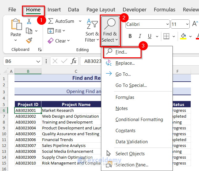
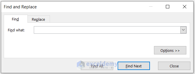
• The “Find and Replace” dialog box will open.

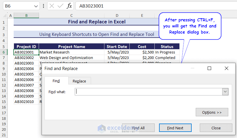
2. Using Keyboard Shortcuts

• Select any cell of the worksheet and press CTRL+F on your keyboard. The Find and Replace dialog box will pop up.
• Enter what you want to find in the ‘Find what’ box and select Find Next to get the result in the worksheet.

Click on the image to get a detailed view

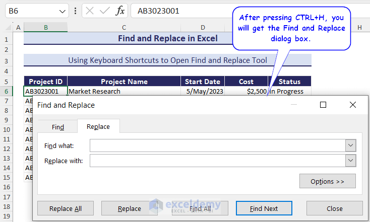
If you want to go to the Replace option, press CTRL+H on your keyboard. Enter what you need to find in the ‘Find what’ box. Enter the data in the ‘Replace what’ box to replace it.

Note: By default, the Find and Replace feature is not case-sensitive, it will find and replace text. However, you can choose the “Match case” option to make it case-sensitive.

How to Fix When Find and Replace Feature in Excel Does Not Work?

There are 6 solutions to fix the problem of Find and Replace feature not working.

1. Ensure cell selection: you must have some value with the finding criteria in your dataset.
2. Unmark Match entire cell contents if the Find and Replace feature is not working.
3. Remove the filter for the proper use of the Find and Replace feature.
4. Delete unwanted spaces in Excel if Find and Replace does not work.
5. If the sheet is protected, remove the protect feature from the sheet to use the Find and Replace tool.
6. You must repair the corrupted Excel worksheet.

How to Find Data in Excel

To find data, you can use the options of the Find & Select feature.

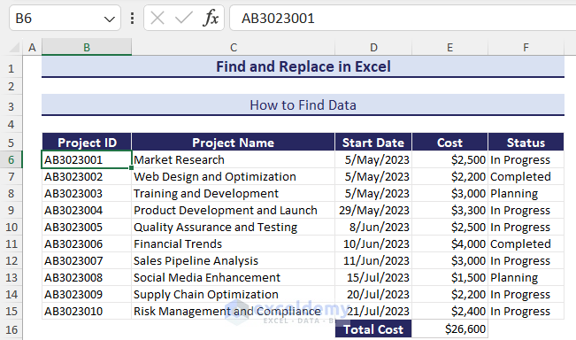
The following sample dataset will be used to illustrate the following examples.

1. Find Text String in Active Excel Sheet

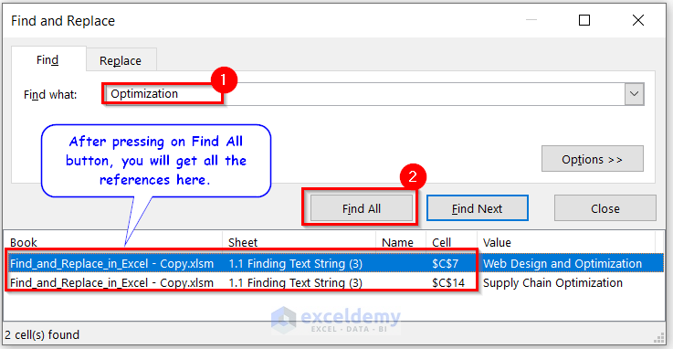
To find any specific text string in a worksheet, input the intended data in the Find What box and press the Find All button in the Find and Replace dialog box. By default, it works on the currently active worksheet.

• Open the Find and Replace dialog box by pressing CTRL+F.
• Enter the text you want to find (e.g. Optimization) in the Find what box >> click the Find All

After clicking the Find All button, all the references will be displayed.

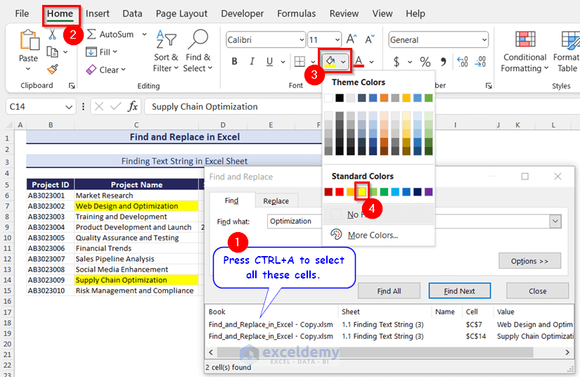
How to Select and Highlight These Texts

• Press CTRL+A to select all these cells in the Find and Replace
• From the Home tab >> go to Font group >> from Fill color drop down, choose any preferable color to highlight these texts.

Click on the image to get a detailed view

2. Find a Cell with Specific Formula

• From Home tab >> Editing group >> Find & Select >> Go To Special.

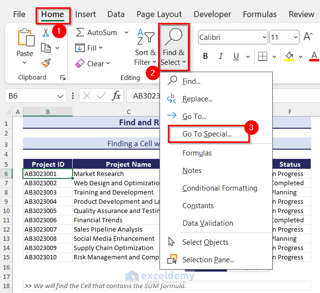
• A dialog box named Go To Special will pop up.
• Select Formulas >> check only the Numbers box >> click OK.

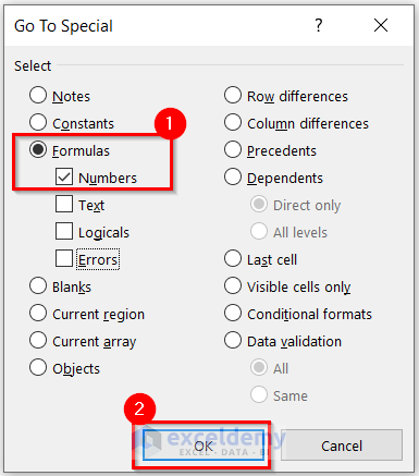
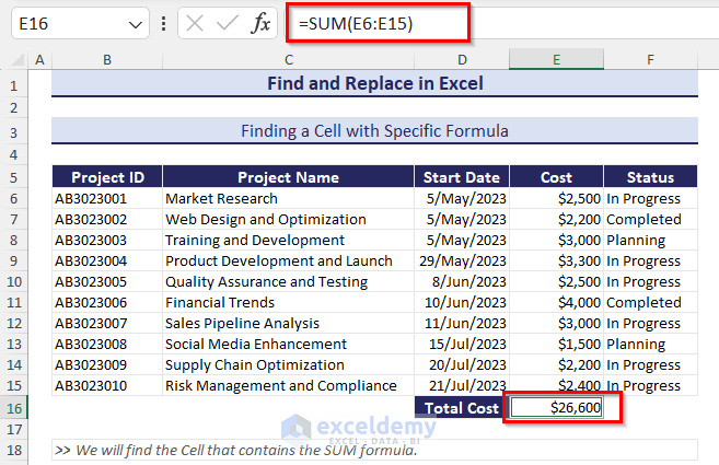
• After searching, the cursor will move to the E16 cell automatically, where the SUM formula is used.

This SUM function returns a numeric value (26,600) as output.

How to Replace Data in Excel

To replace data in a worksheet in Excel, you need to enter the original data (which will be replaced) in the Find what box and then provide the target data in the Replace with box. Press the Replace All button in the Find and Replace box. It will replace all the found data with replaced data within the active worksheet.

Here are 6 examples of how to replace different types of data.

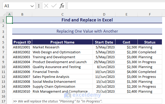
1. Replace One Value with Another

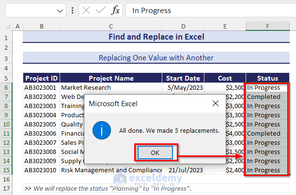
There is a Status column in the sample dataset. This column defines the current status of each project. Let’s assume there are no projects in the planning stage and that all are in progress. We will change the value “Planning” to “In Progress” in the Status column.

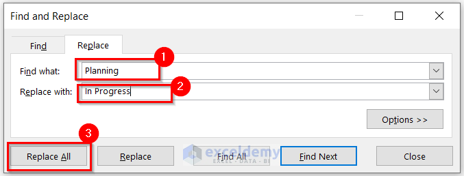
• Press CTRL+H.
• Enter Planning in the Find what box >> enter In Progress in the Replace with box >> press Replace All.

Clicking the Replace All button will find and replace multiple values.

Note: The “Replace All” button replaces all occurrences of the search term at once. Alternatively, you can go through each occurrence using the “Find Next” button and decide to replace or skip each occurrence individually. it’s a good practice to use the “Find Next” button. This prevents unintended replacements.

• You will get an info dialog box where Excel will notify you how many replacements have been made.
• Click OK >> close the Find and Replace window.

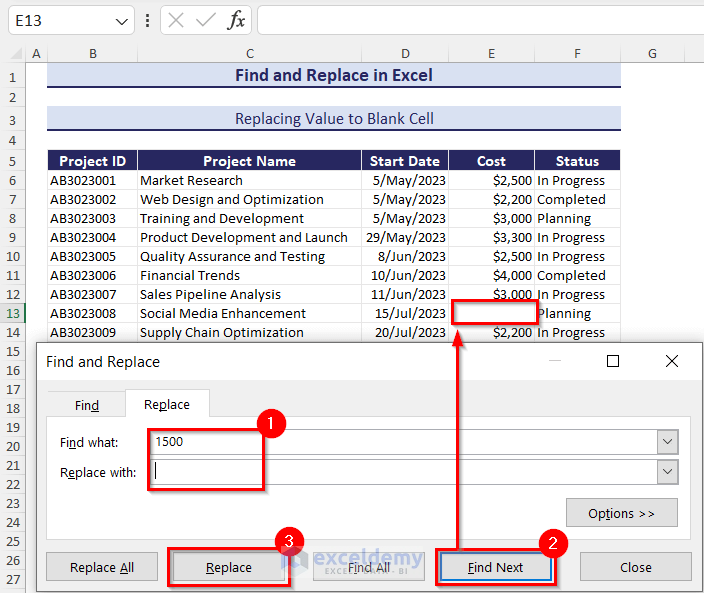
2. Replacing Number to Blank Cell

Suppose we didn’t fix the cost of one project and we want to change that cost ($1500) into a blank cell.

• Press CTRL+H >> enter 1500 in Find what box >> keep the Replace with box blank.
• Click the Find Next button >> this will move your cursor to the E13 cell >> click Replace.

3. Find and Replace Cell Color

We will replace the cell color of cells F7 and F11.

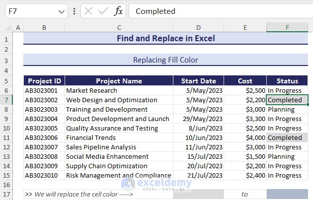
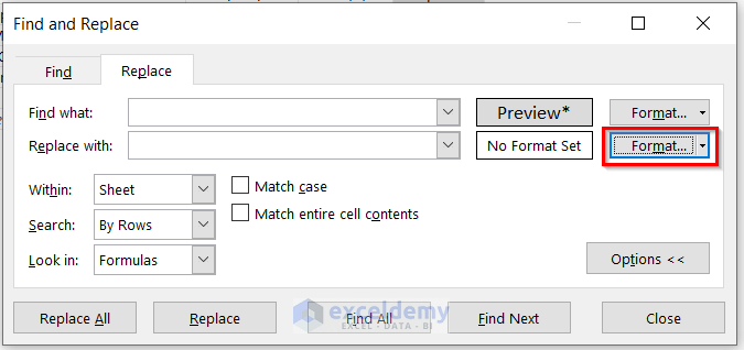
• Press CTRL+H.
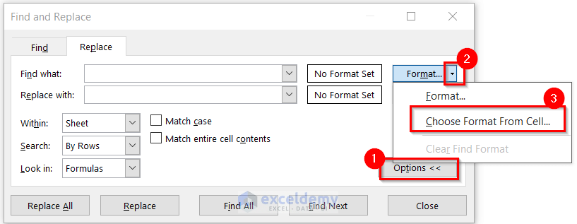
• Click the Options This will open the advanced settings of the Find and Replace tool.
• From the Find what section, click on the Format drop-down menu >> select Choose Format From Cell.

• You will get a dropper >> select the formatted cell with the dropper.

This dropper will consider the format of the F7 cell to find other cells containing a similar format.

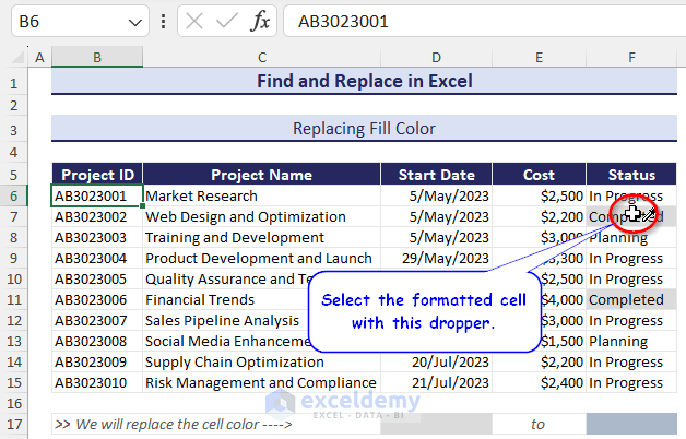
Note: If you don’t use the dropper, you must use the exact format to find the cell.

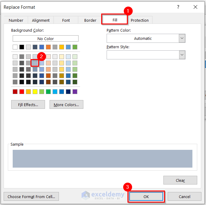
• Set the Fill color that you want to use as a replacement. In the Replace with section, click the Format

• Go to the Fill segment >> choose the Fill color >> click OK.

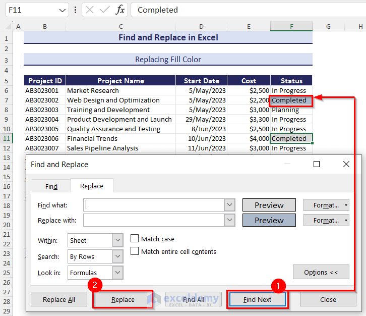
• Click Find Next >> this will move your cursor to the target cell >> click Replace. You have to keep clicking the Find Next >> Replace button until all the required replacements are made.
• Close the Find and Replace dialog box.

Note: You can change the text color using the same procedure. Open Replace Format >> from Font >> change the font Color.

4. Replace Cell References of Formula

Let’s assume that the cell range of summation is E6:E15. We have added some more projects and we want to change the range to E6:E17. To replace cell references in the formula:

• Press CTRL+H.
• Enter the cell index (E15) in Find what box >> Enter the target cell index (E17) in Replace with
• Click Find Next >> Replace.

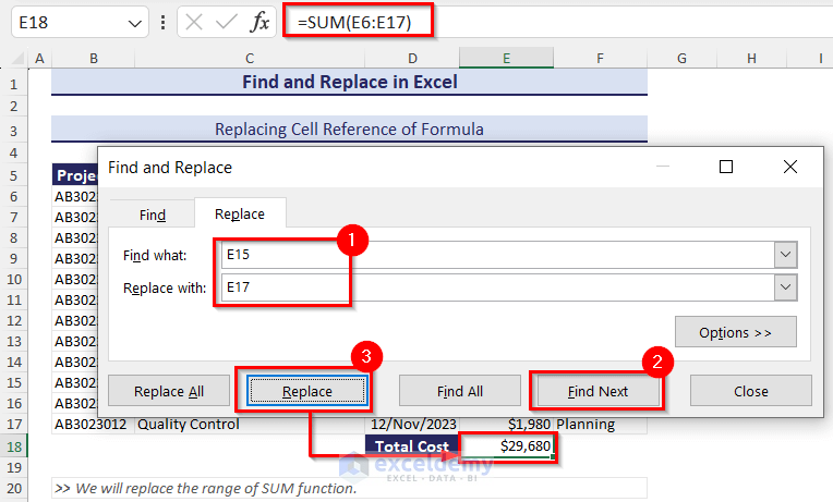
Note: You can change the function as well. In the Find what box, enter the function name (e.g. SUM) and in the Replace with box, enter the required function name (e.g. AVERAGE).

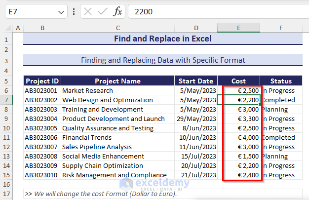
5. Find and Replace Data with Specific Number Format

• We will change the currency format from Dollar to Euro.
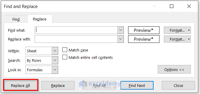
• Press CTRL+H.
• From the Number segment >> go to the Currency category >> choose Euro in the Symbol box >> click OK.

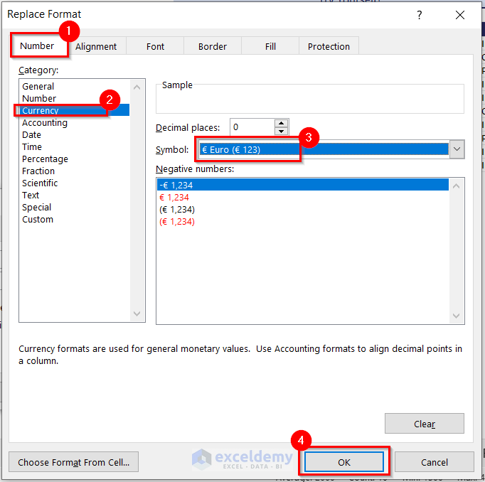
• Click the Replace All button >> click OK >> close the Find and Replace window.

• All the Dollar signs will change to the Euro format.

6. Find and Replace Line Breaks in Excel

There are some line breaks in my dataset. We will to replace these line breaks and use single spaces.

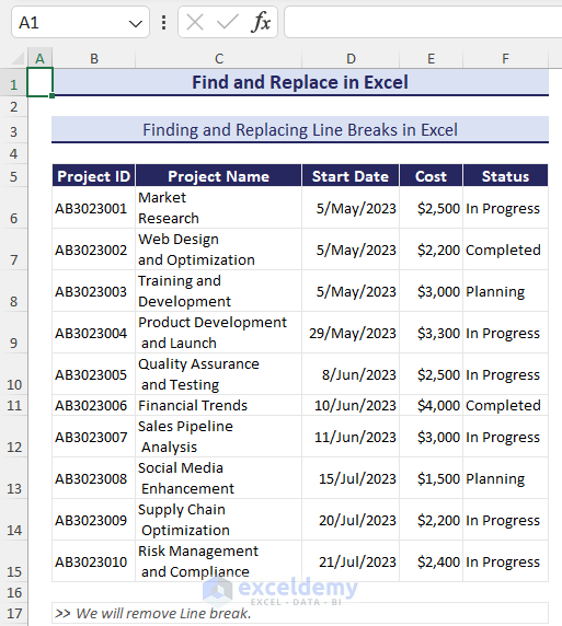
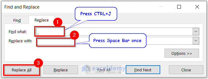
• Go to the Find what box >> press CTRL+J (this will provide a little dot in your box).
• Go to Replace with box >> press Space bar.
• Click Replace All.

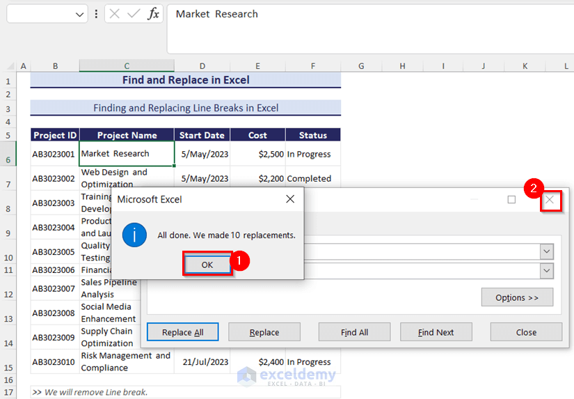
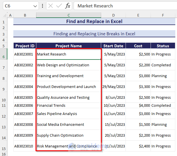
• You will get an info dialog box showing how many replacements have been made>> click OK >> close the Find and Replace window.

Click on the image to get a detailed view

How to Work with Advanced Find and Replace in Excel

To find data within a worksheet or multiple worksheets or even multiple workbooks, you can use the advanced settings of the Find and Replace tool.

1. Find Exact Match Within Entire Workbook – Case Sensitive

We will find the project named ‘Sales Pipeline Analysis’.

• Press CTRL+F >> go to Find what box >> write Sales Pipeline Analysis.
• Click Options >> check the Match entire cell contents.
• Select Workbook in Within box >> click Find All.
• You will get the cell location of Sales Pipeline Analysis.

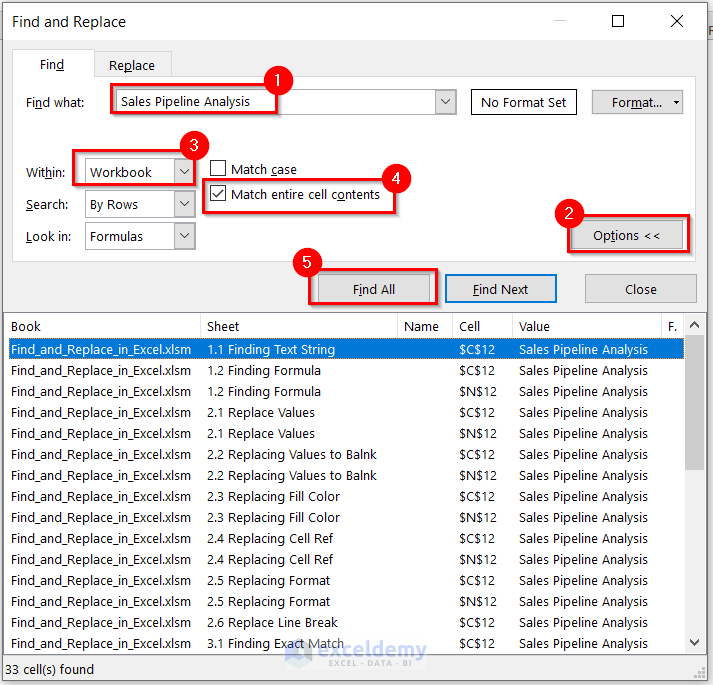
Note: This is case-sensitive. If you write only Sales Pipeline and check the Match entire cell contents box, then you will get a warning from Microsoft Excel saying we couldn’t find what you were looking for. The “Match entire cell contents” option ensures that only complete words are replaced and not partial matches within larger words.

2. Find Comments Within Active Sheet

We have some comments about the projects and we want to find out all the comments as ‘Good’ within the active worksheet.

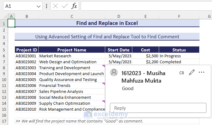
To find a comment within the active worksheet,

Press CTRL+F >> click on Options >> enter Good in the Find what box >> go to the Look in section >> from the drop-down menu, choose Comments >> click Find All.

3. Find Values in Multiple Excel Files

To find values in multiple Excel files,

• Open all the necessary workbooks >> go to any of the workbooks.
• From the Home tab >> under Editing group >> Find & Select >> Find >> enter the data in Find what box >> click Find All.
• This will give all the target data for the active worksheet.
• Don’t close the Find and Replace dialog box.
• Go to another sheet of another workbook >> press Find All. This will give all the target data for that worksheet.
• Similarly, by hovering over different workbooks, you can find the same data on these sheets.

Read More: Find and Replace Values in Multiple Excel Files

How to Find and Replace Data Using Wildcards in Excel

You can use some wildcards, like asterisk and question marks, to find and replace data in Excel. When you know only some characters as the finding criteria, then you can use these wildcards.

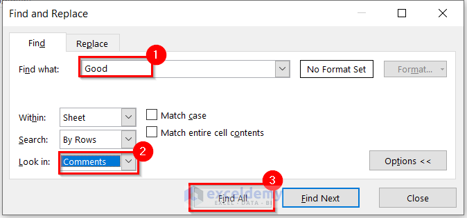
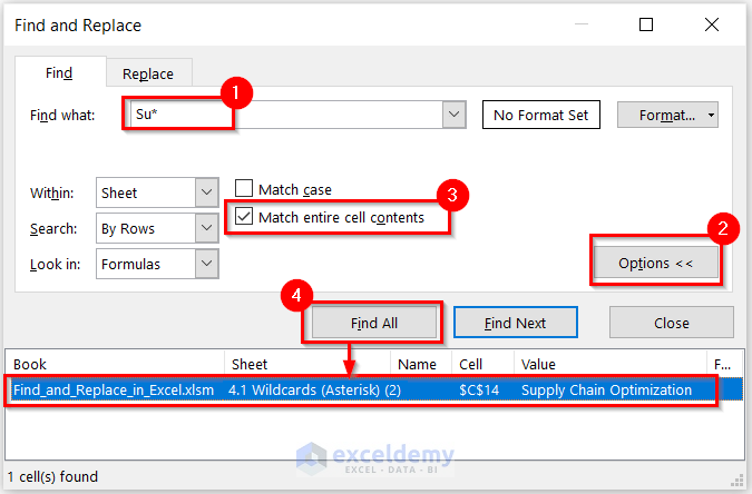
Suppose we want to find all the project names having ‘Su’ as initial characters.

• Press CTRL+F >> enter ‘Su*’ in the Find what box >> click Find All.

This will find all the cell values having ‘Su’ in any position (C10, C14 both). The cell value of C10 is Quality Assurance and Testing, and the cell value of C14 is Supply Chain Optimization.

• To find the project name having ‘Su’ exactly at the first position, then from the Options tab >> check the Match entire cell contents box.
• You will get only the cell value of C14 as output.

If you don’t know a single character of a particular word or term, you can use a question mark to find that entire word/term. For example, we know the ID as A_3023001. But we don’t know the 2nd character of this ID. In this case, we should use the question mark in place of the unknown character.

• Enter A?3023001 in the Find what box >> get all the related IDs (AB3023001, AC3023001, AD3023001).

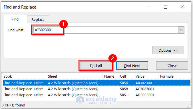
Note:Use question marks in place of unknown characters.

How to Find and Replace Special Characters in Excel

You can replace special characters like asterisks, parentheses, and tabs using the Find and Replace tool.

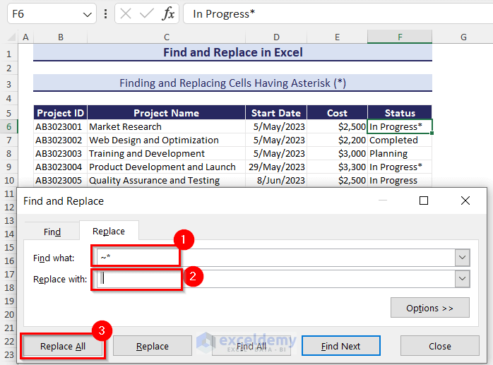
1. Find and Replace Asterisk (*) in Excel

We have an asterisk symbol in the Status column. We will find them and then remove these asterisk marks.

• Press Ctrl+H >>In the Find what box >> enter ~* (use the equivalent symbol first then use an asterisk).
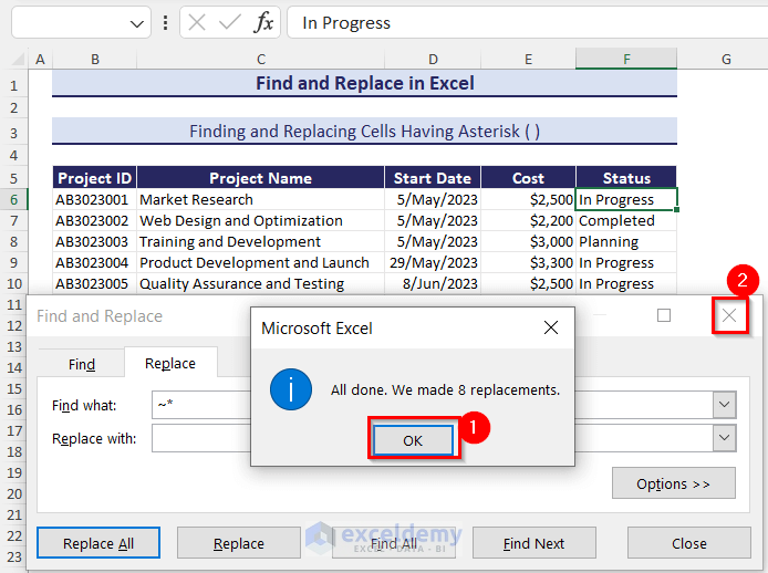
• In the Replace with box >> press Space Bar once >> click Replace All.

This will replace all the asterisks used in the dataset with a single space.

• Click OK >> close the Find and Replace window.
• The output will be shown in the Status column.

To find and remove Tabs, enter Tab in the Find what box >> keep the Replace with box blank >> press Replace All.

Read More: Find and Replace Asterisk (*) Character

2. Removing Cell Values Within Parentheses

We have short codes within parentheses in the Project ID column.

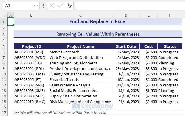
We will remove all these parentheses.

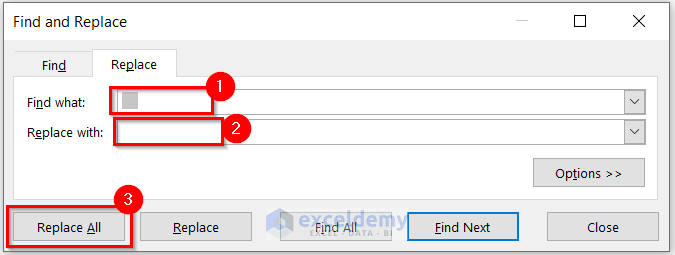
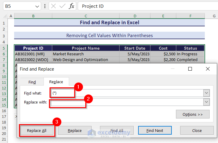
• Press Ctrl+H >> enter (*) in the Find what box >> keep the Replace with box empty.
• Click the Replace All

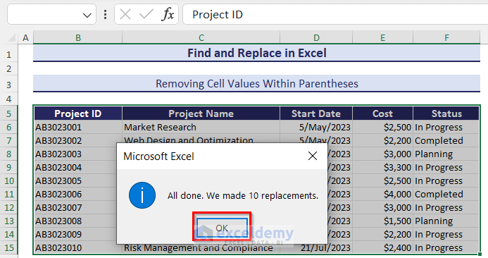
After the replacements, you will see that the short codes are removed from the Project ID column.

Note: If you are making a lot of changes using find and replace, it’s a good idea to create a backup of your Excel file first. This ensures that you can revert to the original data if something goes wrong during the replacement process.

How to Find and Replace with Formulas in Excel

We can use the Excel REPLACE, and SUBSTITUTE functions for the replacement of data. And, we can use the FIND, LOOKUP, VLOOKUP, HLOOKUP, and SEARCH, XLOOKUP functions for looking up values.

1. Using Excel Functions for Replacing Multiple Characters

1.1 Using REPLACE Function to Replace Particular Characters

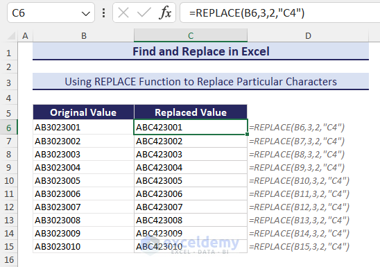
With the REPLACE function, you can replace some specific characters of a string with other characters. The REPLACE function is available from Excel 2007.

In the sample dataset, we have some values in column B. We will replace the particular characters “30” with “C4”.

• Enter the following formula in cell C6.

• Press ENTER.

You will notice that ‘30’ is replaced with ‘C4’.

• Use the Fill Handle tool for the remaining cells.

Read More: Find and Replace Using Formula

1.2 Using SUBSTITUTE Function to Replace Particular Word

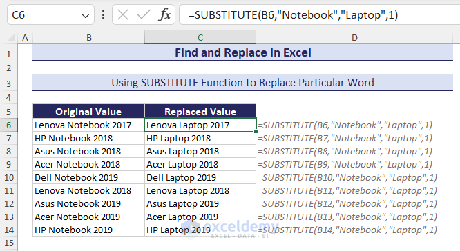
You can use the SUBSTITUTE function to replace a particular word in a string. The SUBSTITUTE function is available from Excel 2007.

In the sample dataset, we will change the word Notebook to Laptop.

• Go to the C6 cell >> enter the following formula:

B6 is the text where the replacement will occur. 1 denotes that the replacement for the entire cell will happen once.

2. Using FIND Function to Find the Position of Specific Characters

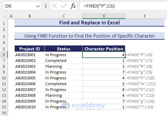
We will use the FIND function to find the position of a specific character “P” within a certain cell.

The FIND function is available from Excel 2007.

• In the D6 cell >> enter the following formula:

You will notice that the character’s position is now shown in cell D6. ‘P’ is found in the C6 cell at the 4th position for the first occurrence.

• We have used the FIND function to find other characters in the remaining cells.

Note: FIND function is case-sensitive. So, you must be careful about sentence cases. However, you can choose multiple characters to find their position.

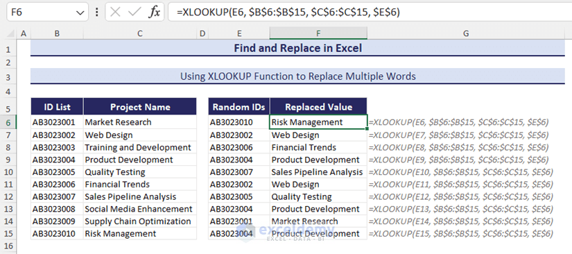
3. Using XLOOKUP Function to Find and Replace Multiple Words from an Excel List

We will find and replace multiple words from an Excel list using the XLOOKUP function. This function is used to look for a value in a range and then return a given value.

You can use this function only in the Excel 365 version.

In the following sample dataset, B6:C15 is the cell range of the list. We will find values using this range as a reference.

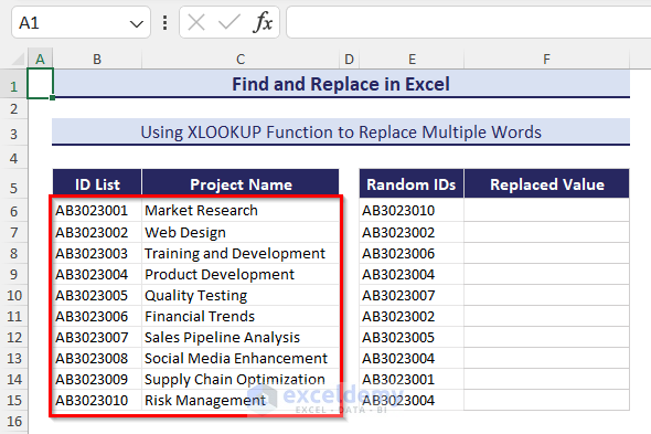
• In cell F6, insert the following formula:

• Press ENTER.
• Use the Fill Handle tool to AutoFill the formula for the remaining cells.

In the XLOOKUP function, we inserted cell E6 as lookup_value, cell range B6:B15 as lookup_array, cell range C6:C15 as return_array and cell E6 as if_not_found.

Click on the image to get a detailed view

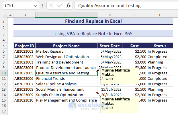
How to Find and Replace Notes in Excel 365 with VBA

The following sample dataset will be used for illustration.

• From the Developer tab >> go to Visual Basic >> Insert >> Module. If you don’t see the Developer tab, then you need to enable the Developer tab.
• Enter the following code in the Module.

Sub ReplaceComments()
Dim ws As Worksheet
Dim cell As Range
Dim comm As comment
Dim searchText As String
Dim replaceText As String
Set ws = ThisWorkbook.Worksheets("Replacing Comment VBA")
searchText = "Rework"
replaceText = "Reworked-OK"
For Each cell In ws.UsedRange.Cells
If Not cell.comment Is Nothing Then
Set comm = cell.comment
If InStr(1, comm.Text, searchText, vbTextCompare) > 0 Then
comm.Text Text:=Replace(comm.Text, searchText, replaceText, , , vbTextCompare)
End If
End If
Next cell
Set comm = Nothing
Set cell = Nothing
Set ws = Nothing
MsgBox "Comments replaced successfully.", vbInformation
End Sub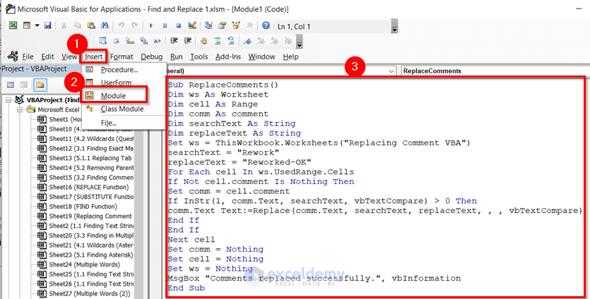

Click on the image to get a detailed view

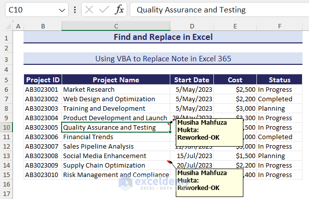
• Press the F5 key to run the code.
• After pressing the Run command, we can see that all the note text that was ‘Rework’ has been replaced with ‘Reworked-OK’.

Download Practice Workbook

Find and Replace in Excel: Knowledge Hub

<< Go Back to Learn Excel