In the following dataset, the product codes are invalid because they have some unnecessary ™ characters inside. To replace these characters, we can use the SUBSTITUTE function.
We’ll use:
- The Find and Replace feature
- The Flash Fill feature
- Dedicated Excel functions to replace text strings
- Excel LAMBDA function and a VBA code for a set of specified characters
- A single formula to replace characters based on conditions.
We have also covered how to replace characters that you cannot type and how to replace foreign letters.
In the last section, I have shown how you can replace or remove non-printable characters.
Notes:
- We have used Excel for Microsoft 365 in this tutorial. The LAMBDA function is exclusive to this version only.
- The Flash Fill feature has been available since Excel 2013.
- You can use the rest of the methods in other Excel versions too.
⏷ Use Find & Replace Feature to Replace Special Characters in Excel
⏵Case 1: Replace All Occurrences of a Character
⏵Case 2: Replace a Character with Different Characters Each Time
⏷ Use Flash Fill Feature
⏷ Use Excel Functions to Replace Special Characters
⏷ Formula to Replace Special Characters Based on Conditions
⏷ Use the LAMBDA Function to Replace a Set of Special Characters
⏷ Using VBA to Replace Special Characters
⏷ Replace Characters Which You Cannot Type
⏷ Replace Foreign Letters with English Alphabets
Method 1 – Use Find & Replace to Replace Special Characters in Excel
How to Open Find and Replace Dialog Window?
We can open the Find and Replace dialog box in 2 ways:
- Go to Home, select Editing, then to Find & Select, and pick Replace.
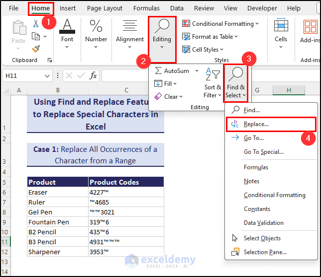
- Press Ctrl + H to directly open up the Find and Replace dialog box.
This feature replaces the values within the cell. If you want to preserve the original data, make sure to back it up.
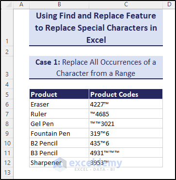
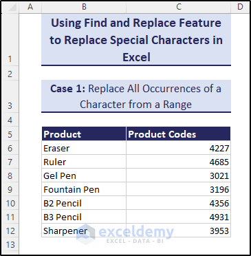
Case 1 – Replace a Character from a Selected Range/Whole Worksheet/Workbook
In the following dataset, there are repeated ™ characters in C6:C12 cells. We are going to replace them with empty strings
Steps:
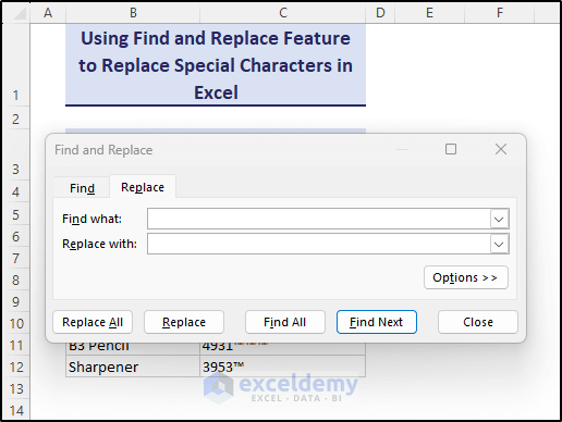
- Open the Find and Replace dialog box.
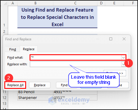
- In the Replace tab of the box, insert ™ in the Find what: field.
- Leave the Replace with: field blank.
- Click on Replace All.
- A message box will pop up indicating the number of replacements that are made. Click OK on it.
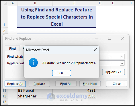
- Close the Find and Replace box after this is over.
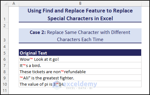
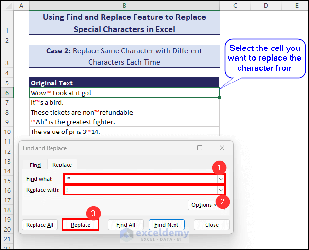
Case 2 – Replace a Character with Different Characters Each Time
To clean the data and make the sentences or words meaningful, we need to replace the ™ characters. But all ™ characters are not replaceable with the same character. For example, Wow™ Look at it go– here ™ is supposed to be replaced by an exclamation mark (!). But in, It™s a bird– here ™ is to be replaced with an apostrophe (‘).
Steps:
- Open up the Find and Replace dialog box.
- Select the first cell with the replaceable value (B6).
- Insert ™ in the Find what field.
- Insert ! in the Replace with field.
- Select Replace.
- The ™ in the first cell will change to !.
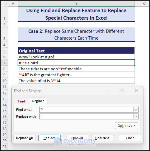
- The selection will automatically shift down. You can also manually change the selection at this point if you want the change to happen in another cell.
- Insert an apostrophe (’) in the Replace with field next and click on Replace.
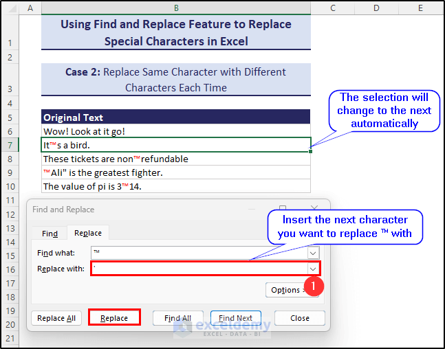
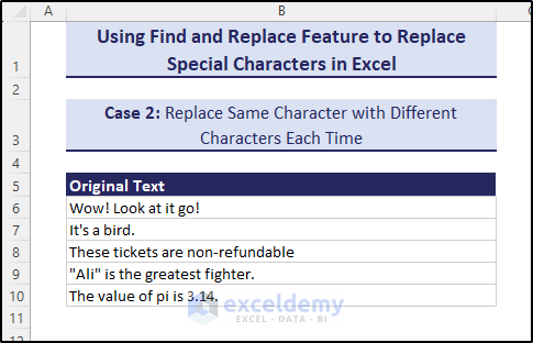
- Repeat this for the rest of the cells and you can get different characters for each cell.
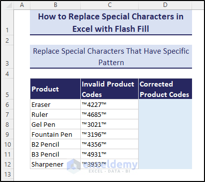
Method 2 – Use the Flash Fill Feature When the Special Characters Maintain a Definite Pattern in Your Data
Excel Flash Fill feature can sense, repeat, and adjust different patterns in a range. If you establish a pattern in the first 2 cells in a range, the Flash Fill tool can follow this pattern and show autofill suggestions for the rest of the cells. The Flash Fill can sense patterns only from a range adjacent to it and the changes must follow a pattern.
The dataset below has the special character ™ at the start and end of every number.
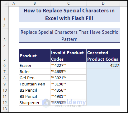
Steps:
- Write the first product code 4227 manually in cell D6, which is adjacent to the source cell C6.
- Start writing the next product code 4685 in cell D7. At this point, the Flash Fill tool will detect the pattern you are establishing and suggest the rest of the values like the image below.
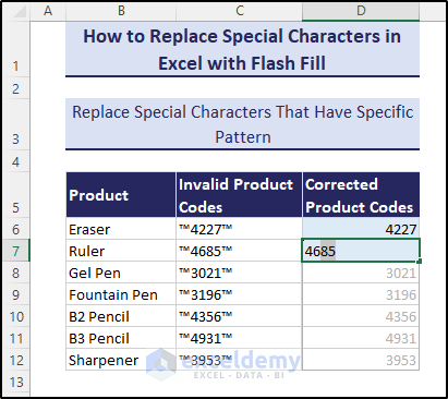
- Press Enter once the suggestion appears.
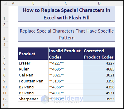
Note:
You can use the keyboard shortcut Ctrl + E to use the Flash Fill feature too. For example, you could insert 4227 as the first cell value and press Ctrl + E. It should give the exact same result.
Read More: Find And Replace Multiple Values in Excel
Method 3 – Use Excel Functions to Replace Special Characters in Excel in Different Cases
Case 3.1 – Use SUBSTITUTE Function Once When the Replaceable Character Is Same in All Cells
The syntax of the SUBSTITUTE function is:
=SUBSTITUTE(text, old_text, new_text, [instance_num])
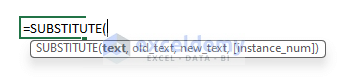
To replace a special character, we need to insert the replaceable character in the second argument.
Let’s take the following dataset. All the invalid product codes have some unnecessary ™ characters
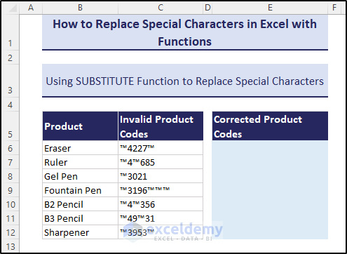
- We are going to replace ™ with empty strings using this function like the following:
=SUBSTITUTE(C6,"™","")
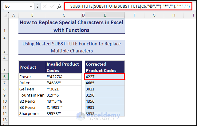
Case 3.2 – Use Nested SUBSTITUTE functions to Replace Multiple Special Characters
If there is more than one character you want to replace, we can nest multiple SUBSTITUTE functions. Let’s take a dataset like below which contains three special characters ™, ©, and ®.
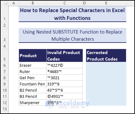
- Nest 3 SUBSTITUTE functions like this below:
=SUBSTITUTE(SUBSTITUTE(SUBSTITUTE(C6,"©",""),"®",""),"™","")
Note:
This method is not suitable when there are a lot of different characters to replace.
Read More: How to Substitute Multiple Characters in Excel
Case 3.3 – Use the REPLACE Function to Replace Special Characters Wholly or Partially from a Certain Position
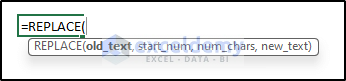
The syntax of the REPLACE function is as follows:
=REPLACE(old_text, start_num, num_chars, new_text)
Here, you have to specify the cell, i.e., old_text, where the replaceable text lies. Then input start_num, i.e., from which position in the string, the replacement will start. Then specify num_chars i.e., the number of characters to be replaced by new_text in the 4th argument.
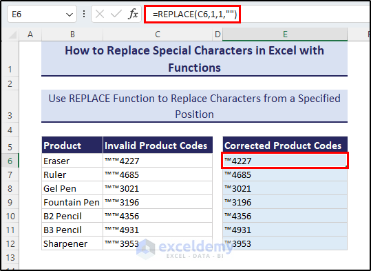
In the following dataset, we have 2 ™ characters in each product code. We want to keep one ™ and replace the other one with an empty string.
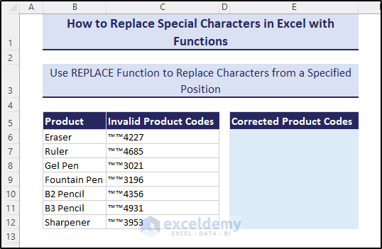
- Use the following formula for that:
=REPLACE(C6,1,1,"")
Method 4 – Use a Formula That Can Replace Special Characters Based on Conditions
Let’s keep only the numbers in the product codes, while the rest of the characters will be replaced.
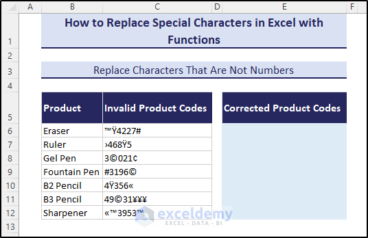
The character codes of digits in Excel are 48 through 57.
We will replace characters with codes lower than 48 and greater than 57.
- Go to cell E6 and insert the following formula, then copy it for the rest of the cells:
=TEXTJOIN("",TRUE,IF(((CODE(MID(C6,SEQUENCE(LEN(C6)),1)))<=57*(CODE(MID(C6,SEQUENCE(LEN(C6)),1))>=48))*1,MID(C6,SEQUENCE(LEN(C6)),1),REPLACE(MID(C6,SEQUENCE(LEN(C6)),1),1,1,"")))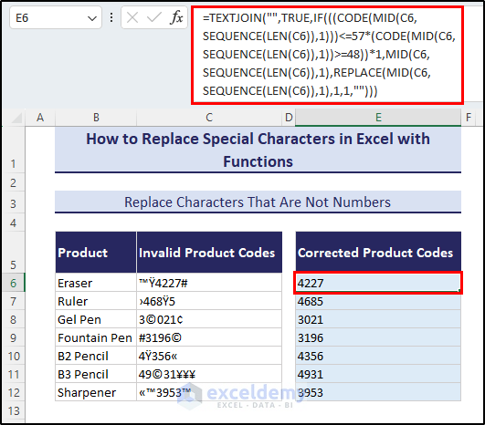
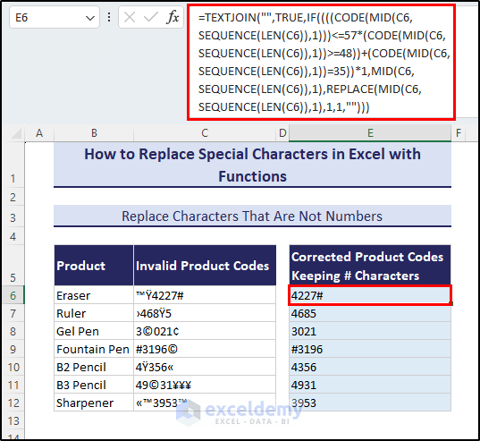
- If you want to add more conditions, i.e., remove characters that are not numbers, but keep “#” characters, the formula will be:
=TEXTJOIN("",TRUE,IF((((CODE(MID(C6,SEQUENCE(LEN(C6)),1)))<=57*(CODE(MID(C6,SEQUENCE(LEN(C6)),1))>=48))+(CODE(MID(C6,SEQUENCE(LEN(C6)),1))=35))*1,MID(C6,SEQUENCE(LEN(C6)),1),REPLACE(MID(C6,SEQUENCE(LEN(C6)),1),1,1,"")))Here, CODE(MID(C6,SEQUENCE(LEN(C6)),1))=35 condition is used to keep the # characters (35 is the character code of #).
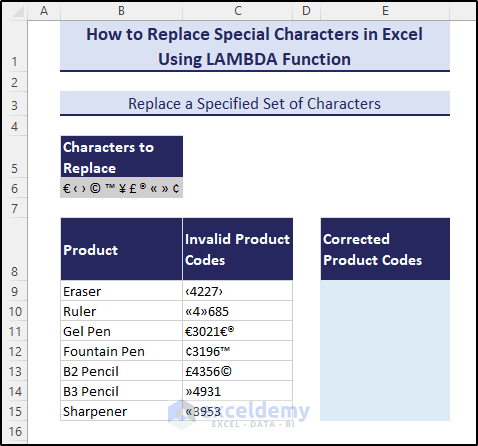
Method 5 – Use the LAMBDA Function to Replace a Set of Special Characters at Once
The LAMBDA function can allow us to create custom functions that can replace multiple characters with a single formula. Here is a dataset like that. The characters we want to remove are in cell B6.
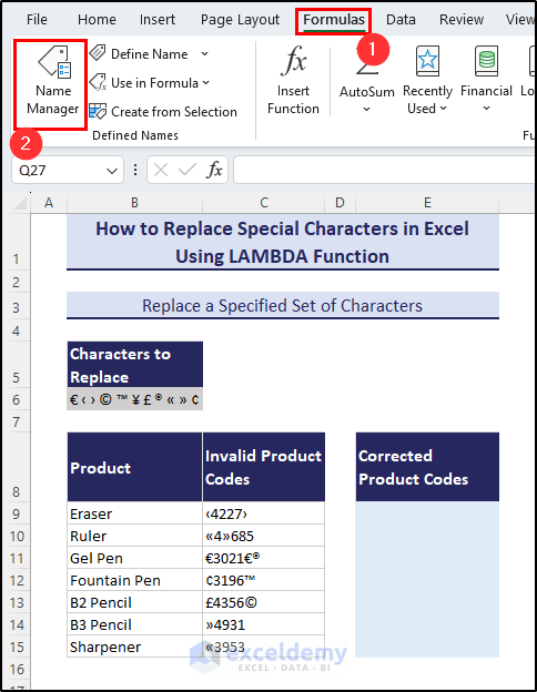
- Go to the Formulas tab in the ribbon and select Name Manager.
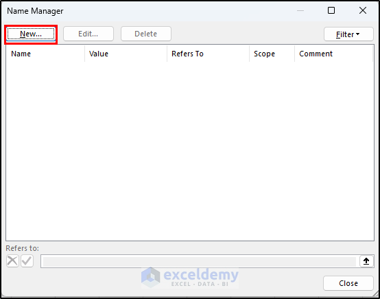
- Select New in the Name Manager box.
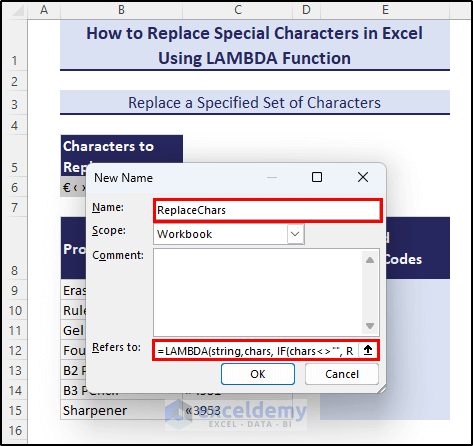
- Another box will pop up called New Name. Select a name in the Name field. We named it ReplaceChars.
- In the Refers to field, use this formula:
=LAMBDA(string,chars, IF(chars<>"", ReplaceChars(SUBSTITUTE(string, LEFT(chars, 1), ""), RIGHT(chars, LEN(chars) -1)), string))
- Close both the boxes.
- Go back to the spreadsheet and use the formula below:
=ReplaceChars(C9,$B$6)
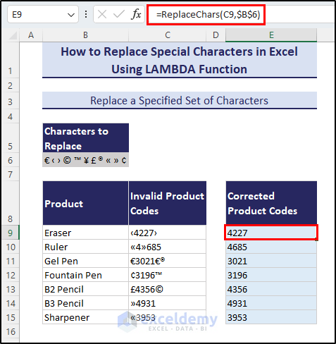
This way, the function will now remove all of the characters that are in the B6 cell.
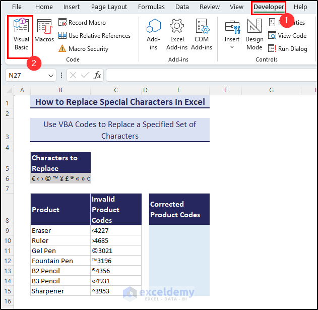
Method 6 – Using VBA to Replace Special Characters
- Select Developer tab (enable the Developer tab on your ribbon) and go to Visual Basic.
- In the VBA window, select Insert and pick Module.
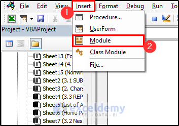
- Insert the following code in the module:
Function ReplaceUnwantedChars(str As String, chars As String)
  For index = 1 To Len(chars)
    str = Replace(str, Mid(chars, index, 1), "#")
  Next
  ReplaceUnwantedChars = str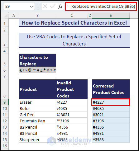
End Function- Close the window and use this function in the spreadsheet:
=ReplaceUnwantedChars(C9,$B$6)
How to Replace Characters Which You Cannot Type in Excel
There are some invisible characters or some you can’t copy in Excel. We can use the CODE and CHAR functions in these cases to replace them.
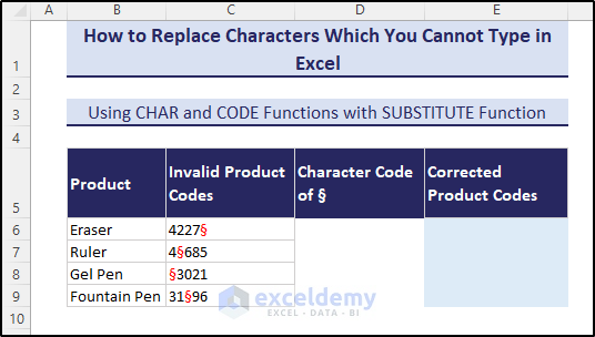
- We can find the character code for § by using the following formula.
=CODE(RIGHT(C6))
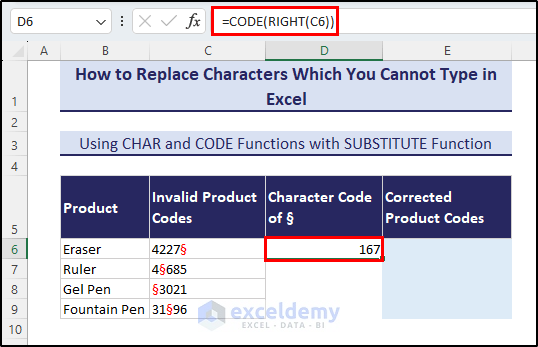
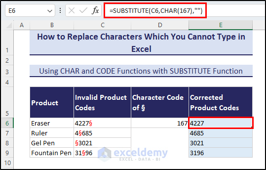
The result gives us 167. So, using CHAR(167) will return the character §.
- Use the following formula to remove the character from the product codes.
=SUBSTITUTE(C6,CHAR(167),"")
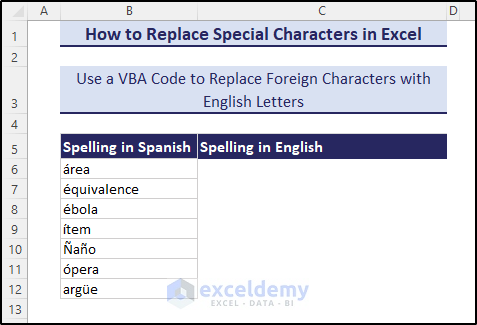
How to Replace Foreign Letters with English Ones in Excel
Let’s take a sample dataset with Spanish words that have the same spelling as English.
- Open a new module in the VBA window and insert the following code in it:
Function AccReplace(CellVal As String)
Dim Esp As String * 1
Dim Eng As String * 1
Dim i As Integer
Const EspChars = "ŠŽšžŸÀÁÂÃÄÅÇÈÉÊËÌÍÎÏÐÑÒÓÔÕÖÙÚÛÜÝàáâãäåçèéêëìíîïðñòóôõöùúûüýÿ"
Const EngChars = "SZszYAAAAAACEEEEIIIIDNOOOOOUUUUYaaaaaaceeeeiiiidnooooouuuuyy"
For i = 1 To Len(EspChars)
Esp = Mid(EspChars, i, 1)
Eng = Mid(EngChars, i, 1)
CellVal = Replace(CellVal, Esp, Eng)
Next
AccReplace = CellVal
End Function
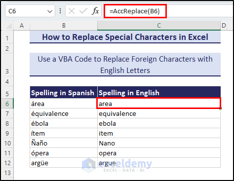
- Go back to the sheet and use the formula below:
=AccReplace(B6)
Download the Practice Workbook
Related Articles
- How to Find and Replace Asterisk (*) Character in Excel
- Find and Replace Tab Character in Excel
- [Fixed!] Excel Find and Replace Not Working
- How to Find and Replace in Excel Column
<< Go Back to Find and Replace | Learn Excel
Get FREE Advanced Excel Exercises with Solutions!
