Inserting dates in Excel can be used for a variety of purposes, including data tracking and date-time calculations. In this article, we are going to show you seven suitable ways to insert a date in Excel. So, let’s start this article and explore these methods.
How to Insert Date in Excel: 7 Suitable Methods
In this section of the article, we will discuss seven effective methods to insert a date in Excel. Not to mention, we used the Microsoft Excel 365 version for this article; however, you can use any version according to your preference.
1. Using Keyboard Shortcuts
Using the keyboard shortcut is the easiest way to insert a date in Excel. Here, we will demonstrate two separate keyboard shortcuts. So, let’s follow the steps mentioned below.
Steps:
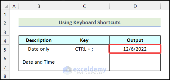
- Firstly, select cell D5 and use the keyboard shortcut CTRL + ;. This will give you the current date in cell D5.
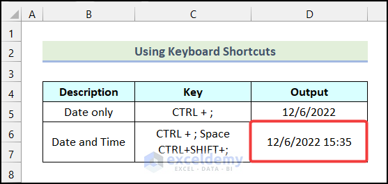
- Now, if you want to have the current date and time together in a cell, then press the keyboard shortcut CTRL + ; first to insert the current date.
- Then, press SPACE key.
- After that, use another keyboard shortcut CTRL + SHIFT + ;.
Consequently, you will have the current date and time together in cell D5, as shown in the following image.
2. Applying Volatile Date & Time Functions
Excel provides several built-in functions to insert dates. Here, we will use the TODAY and NOW functions of Excel to insert a date.
2.1 Using TODAY Function
The TODAY function is one of the most commonly used functions in Excel. Let’s use the steps outlined below to use the TODAY function to insert a date in Excel.
Steps:
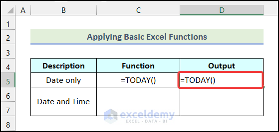
- Firstly, use the following formula in cell D5.
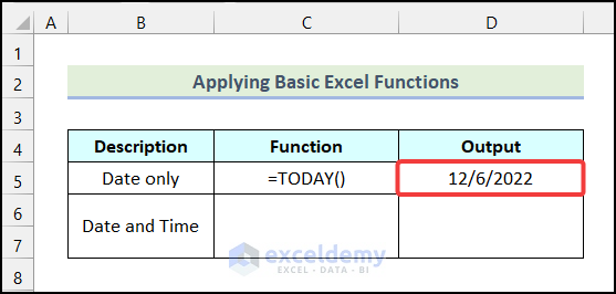
=TODAY()- Following that, press ENTER.
As a result, you will have the date of present-day in cell D5.
2.2 Utilizing NOW Function
The NOW function provides us with not only today’s date but also the current time. Let’s follow the steps given below.
Steps:
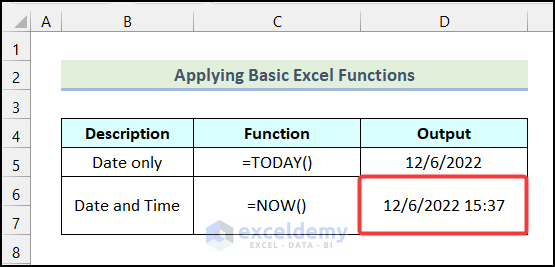
- Firstly, apply the formula given below in cell D6.
=NOW()- After that, hit ENTER.
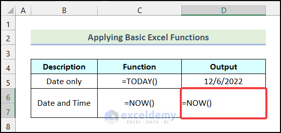
Subsequently, you have the current date and time in cell D6, as shown in the image below.
3. Using DATE Function
To insert dates, we can use another function called the DATE function. It creates a valid date by combining the components year, month, and day. Let’s follow the steps mentioned below.
Steps:
- Firstly, insert the following formula in cell D5.
=DATE(2021,9,28)Here, 2021 is the year, 9 and 28 are the month and day respectively.
- Then, press ENTER.
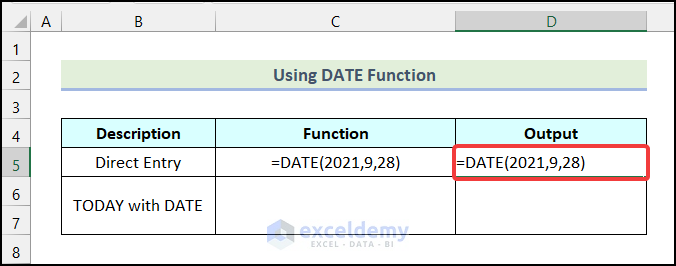
Consequently, you will find the specified date in cell D5.

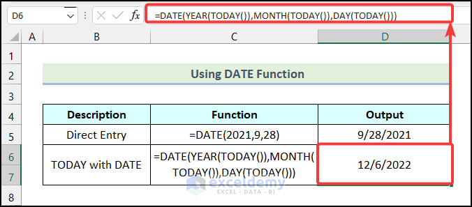
To insert dates, we can combine the DATE function with the TODAY function. The formula will be in such a way that DATE function will fetch the year, month, and day produced from the TODAY function.
- Firstly, use the following formula in cell D6.
=DATE(YEAR(TODAY()),MONTH(TODAY()),DAY(TODAY()))Formula Breakdown
- The YEAR function fetches the year value from the result of the TODAY function.
- Output → 2022.
- The MONTH function fetches the month value from the result of the TODAY function.
- Output → 12.
- The DAY function fetches the day value from the result of the TODAY function.
- Output → 6.
- Finally, DATE(YEAR(TODAY()),MONTH(TODAY()),DAY(TODAY())) → It becomes DATE(2022,12,6).
- Output → 12/6/2022.
- Now, press ENTER.
As a result, you will have today’s date in cell D6, as demonstrated in the following picture.
4. Utilizing AutoFill Feature
The AutoFill feature is a quite simple yet powerful feature of Excel. We can use the AutoFill option to automatically fill out dates.
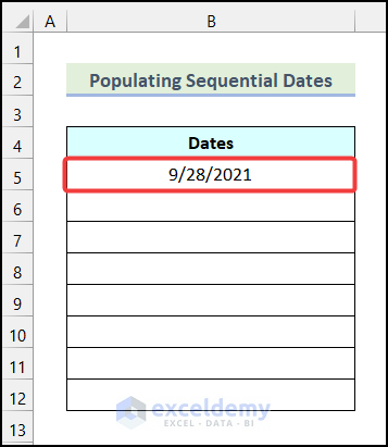
4.1 Populating Sequential Dates
First, we will discuss how we can populate dates sequentially using the AutoFill option. Let’s use the steps mentioned below to do this.
Steps:
- Firstly, enter any date you want in cell B5.
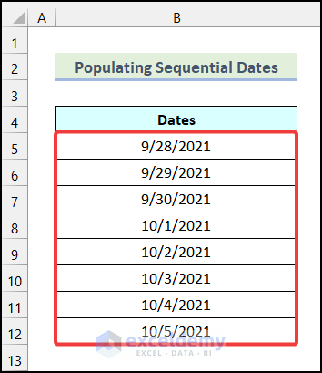
- Then, drag the Fill Handle up to cell B12, and the empty cells will be populated with sequential dates.
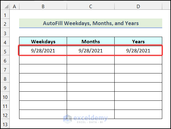
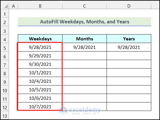
4.2 AutoFill Weekdays, Months, and Years
Suppose you want to have only the Weekdays in your worksheet. To achieve this, let’s use the steps outlined below.
Steps:
- Firstly, enter any date you want in the first row, as shown in the following image.
- After that, drag the Fill Handle up to cell B12.
- Then, click on the AutoFill options button.
- Next, choose the Fill Weekdays option from the drop-down.
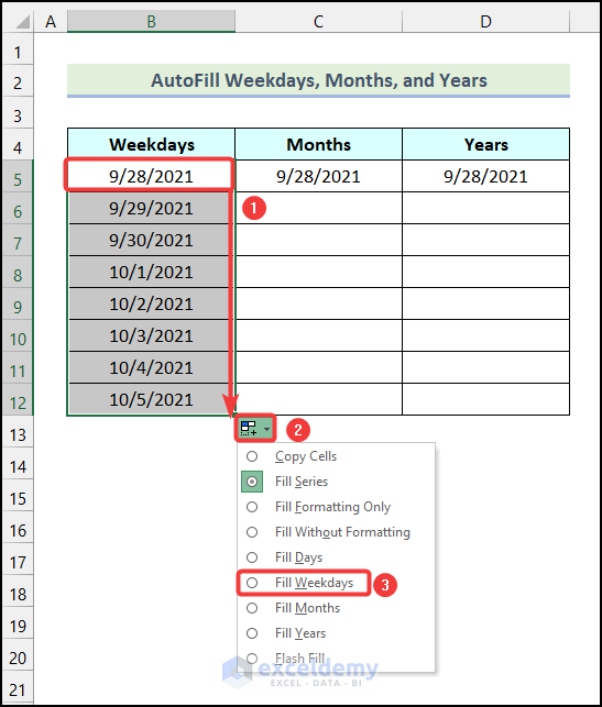
As a result, you will have a list of only workdays as shown in the image below.
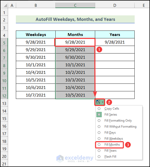
Now, let’s say we need to change only the Month from the date. Day and Year will remain the same.
- Firstly, select cell C5 and drag the Fill Handle up to cell C12.
- Then, click on the AutoFill Options button.
- After that, select the Fill Months option from the drop-down.
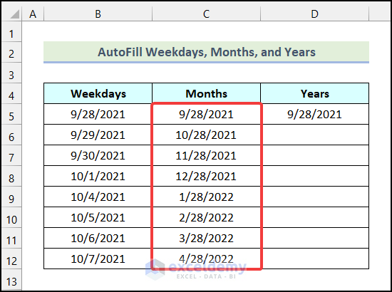
Subsequently, you will have the following output on your worksheet.
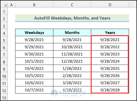
You can also change only the Years while keeping the Day and the Month the same. To do this, let’s follow the procedure mentioned below.
- Firstly, select cell D5 and drag the Fill Handle up to cell D12.
- Then, click on the AutoFill Options button.
- Finally, choose the Fill Years option from the drop-down.
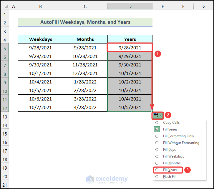
As a result, you have a list of dates with only the years changing incrementally.
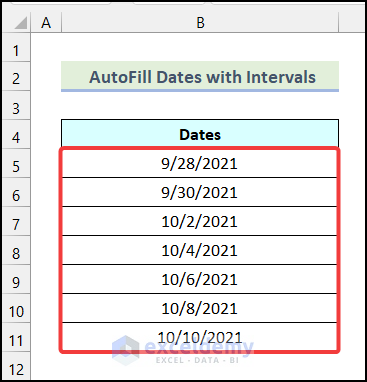
4.3 AutoFill Dates with Intervals
In the earlier section, we have auto-filled dates without any intervals. If you want dates after a regular interval, then follow the instructions outlined in the following section.
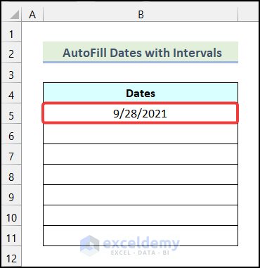
Steps:
- Firstly, enter any date you want in cell B5, as shown in the following picture.
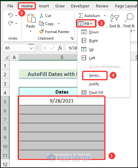
- After that, select all the cells in which you want to have the dates.
- Then, go to the Home tab from the Ribbon.
- Now, click on the Fill option from the Editing group.
- Following that, choose the Series option from the drop-down.
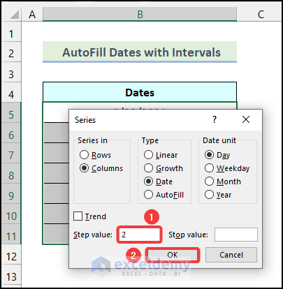
- Now in the Series dialogue box, type 2 inside the Step value field. This means in the output we will get dates after every two days. You can enter different Step value according to your requirement.
- Then, click OK.
As a result, you will get the following output on your worksheet as demonstrated in the following picture.
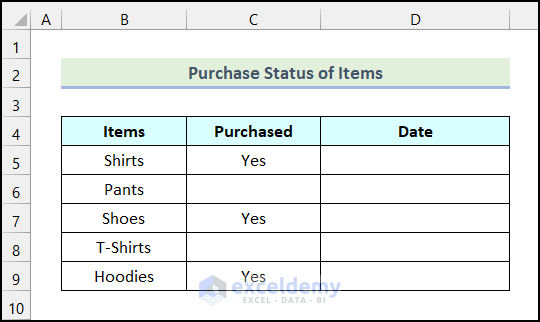
5. Inserting Date Depending on Adjacent Cell
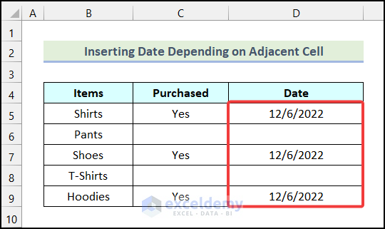
In Excel, we can form a formula that will help us insert dates depending on the adjacent cell. Here, we will use the IF function to develop a condition based on which a date will be inserted in an adjacent cell. Let’s say, we have the Purchase Status of Items as our dataset. We will insert a date in the Date column based on purchase status. Now, let’s use the steps mentioned below to do this.
Steps:
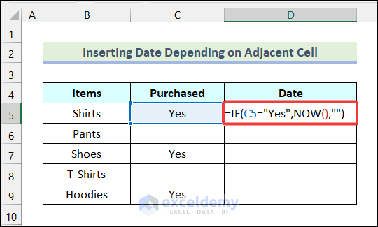
- Firstly, use the following formula in cell D5.
=IF(C5="Yes",NOW(),"")Here, cell C5 indicates the purchase status for Shirts.
Formula Breakdown
- Here, the NOW() function returns the current date and time.
- In the IF function,
- C5=”Yes” → This is the logical_test argument.
- NOW() → This indicates the [value_if_true] argument.
- “” → It refers to the [value_if_false] argument.
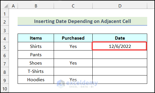
- Output → 12/6/2022.
- Now, press ENTER.
Consequently, you will have the following output in cell D5 as shown in the following image.
- Finally, use the AutoFill option of Excel to get the rest of the outputs.
Read More: How to Insert Day and Date in Excel
6. Updating Date-Time upon Changes in Adjacent Cell
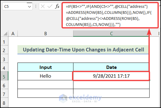
We can construct a formula that will insert and update dates (and times) whenever we update the adjacent cell in Excel. Here, we will use the ADDRESS, and CELL functions to create the formula. The ADDRESS function returns the address for a cell based on a given ROW and COLUMN number and the CELL function returns information about a cell in a worksheet. Now, let’s follow the steps mentioned in the following section.
Steps:
- Firstly, use the following formula in cell C5.
=IF(B5<>"",IF(AND(C5<>"",@CELL("address")=ADDRESS(ROW(B5),COLUMN(B5))),NOW(),IF(@CELL("address")<>ADDRESS(ROW(B5),COLUMN(B5)),C5,NOW())),"")Here, cell B5 indicates the first cell of the Input column, and cell C5 represents the first cell of the Date column.
Formula Breakdown
- Firstly, let’s see the outputs of the following functions to simplify our formula.
- @CELL(“address”) → “$C$5”.
- ADDRESS(ROW(B5),COLUMN(B5)) → {“$B$5”}.
- Now, the formula becomes → =IF(B5<>””,IF(AND(C5<>””,”$C$5″={“$B$5”}),NOW(),IF(“$C$5″<>{“$B$5″},C5,NOW())),””).
- Here, inside the second IF function,
- AND(C5<>””,”$C$5″={“$B$5”}) → It represents the logical_test argument.
- In the AND function,
- C5<>”” → It is the logical1 argument.
- “$C$5″={“$B$5”} → This represents the [logical2] argument.
- Output → FALSE.
- NOW() → It is the [value_if_true] argument.
- IF(“$C$5″<>{“$B$5”},C5,NOW()) → This refers to the [value_if_false] argument.
- Inside this IF function,
- “$C$5″<>{“$B$5”} → It is the logical_test argument.
- C5 → This is the [value_if_true] argument.
- NOW() → It is the [value_if_false] argument.
- Output → 44467.7201388889. This represents the current date and time in numerical format.
- Output → 44467.7201388889.
- AND(C5<>””,”$C$5″={“$B$5”}) → It represents the logical_test argument.
- Now, the formula becomes → =IF(B5<>””,{44467.7201388889},””).
- B5<>”” → This is the logical_test argument.
- {44467.7201388889} → It is the [value_if_true] argument.
- “” → This refers to the [value_if_false] argument.
- Output → {44467.7201388889}. Which is 9/28/2021 17:17 in date format.
- After that, press ENTER.
As a result, you will have the date and time of the last change in cell B5 inside cell C5.
- Finally, use the AutoFill option of Excel to obtain the rest of the outputs as demonstrated in the following image.

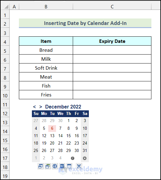
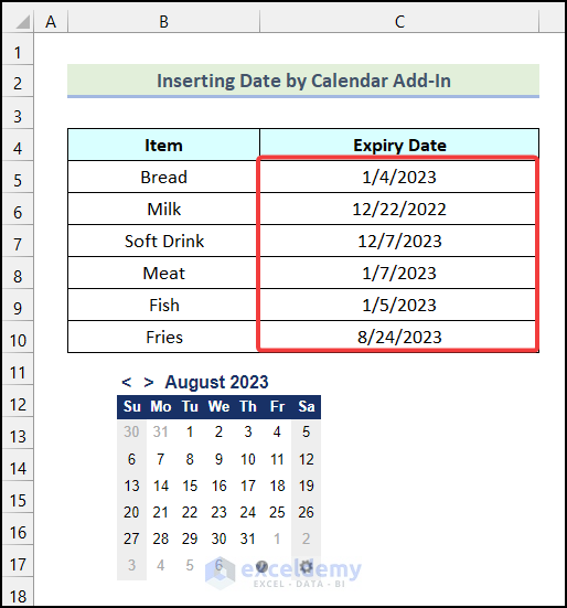
7. Inserting Date by Calendar Add-in
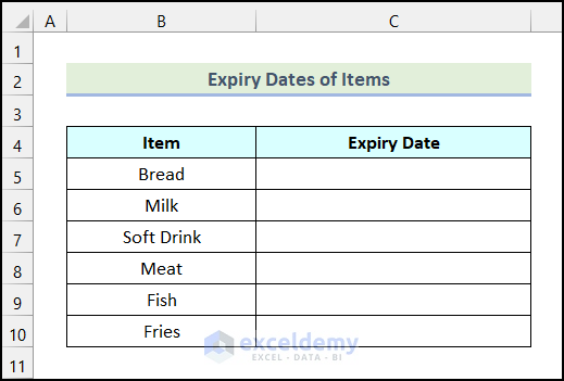
In Excel, we can use lots of free Add-ins provided by Microsoft. In this method, we are going to use one of the Calendar Add-ins. Let’s say, we have the Expiry Dates of Items as our dataset. Our goal is to insert the date in the Expiry Date column using the calendar add-in.
Steps:
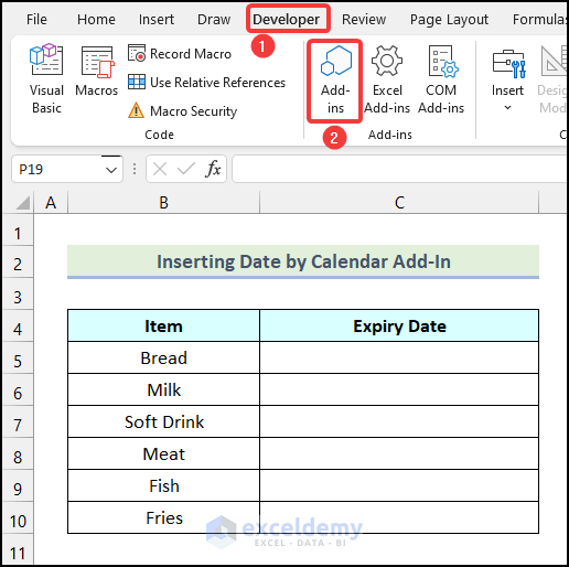
- Firstly, go to the Developer tab from Ribbon.
- Then, click on the Add-ins option from the Add-ins group.
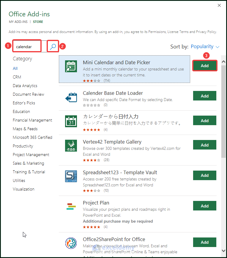
As a result, the Office Add-ins dialogue box will open on your worksheet.
- Now, in the Office Add-ins dialogue box, search for “calendar”.
- Then, find the Mini Calendar and Date Picker add-in from the list.
- After that, click on the Add option.
- Following that, a pop-up window will appear. Then, click on Continue.

Consequently, a calendar will be added to your worksheet, as shown in the following image.
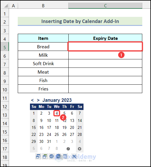
- Now, to insert a date in a cell, first select the cell in which you want to enter the date. In this case, we selected cell C5.
- Then, click on your preferred date from the calendar.
As a result, your selected date will appear in cell C5.
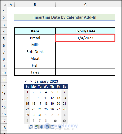
- Follow, the same procedure and you will be able to insert dates in the remaining cells as shown in the picture below.
How to Insert Date in Excel Formula
In this section of the article, we will learn how we can insert a date inside an Excel formula. To do this, let’s follow the instructions outlined below.
Steps:
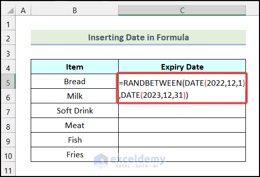
- Firstly, enter the formula given below in cell C5.
=RANDBETWEEN(DATE(2022,12,1),DATE(2023,12,31))Formula Breakdown
- Here, in the RANDBETWEEN function,
- DATE(2022,12,1) → It is the bottom argument.
- DATE(2023,12,31) → This refers to the top argument.
- Now, the RANDBETWEEN function will return a random date between the bottom and top date.
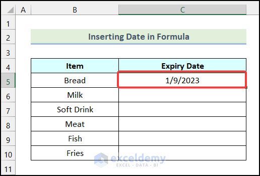
- Output → 1/9/2023.
- Following that, hit ENTER.
Consequently, you will have the following output in cell C5.
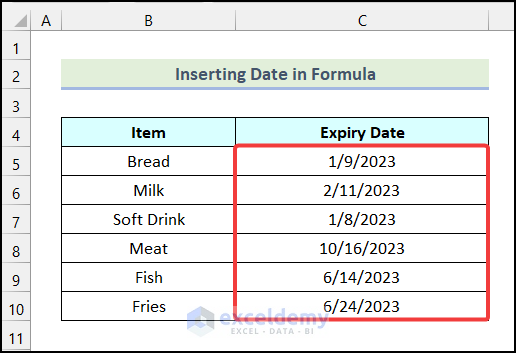
- Lastly, use Excel’s AutoFill option to get the rest of the Expiry Dates as shown in the following picture.
You can also follow various approaches to Insert Date in Excel Formula.
Practice Section
In the Excel Workbook, we have provided a Practice Section on the right side of the worksheet. Please practice it yourself.
Download Practice Workbook
Conclusion
So, these are the most common and effective methods you can use anytime while working with your Excel datasheet to insert date in Excel. If you have any questions, suggestions, or feedback related to this article, you can comment below.
How to Insert Date: Knowledge Hub
<< Go Back to Date-Time in Excel | Learn Excel
Get FREE Advanced Excel Exercises with Solutions!
