Sometimes you need to skip every other column in Excel. Using Excel Formulas, you can do such a job in a few moments. In this article, we will show the Excel formula to skip every other column. I hope you find this article interesting and understand lots of Excel formulas.
How to Skip Every Column Using Excel Formula: 3 Suitable Methods
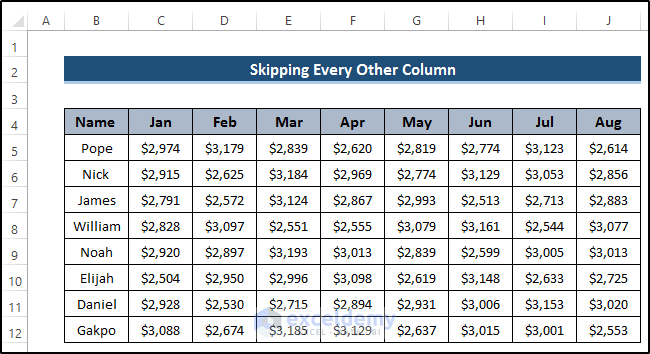
To skip every column in the Excel formula, we have found three different methods through which you can do the job perfectly. In these three methods, we utilize several Excel functions and a VBA code. All these three methods are fairly effective to use and also user-friendly. To show all the methods, we take a dataset that includes some salesman name and their sales amount over several months.
1. Combination of MOD, COLUMN and SUMPRODUCT Functions
Our first method to skip the other column in the Excel formula is by using the combination of MOD, COLUMN, and SUMPRODUCT functions. In this method, at first, we would like to select the columns in which you find the sum value using MOD and COLUMN functions. After that, the SUMPRODUCT function finds the required summation of those columns skipping the other columns. To understand the method properly, follow the steps.
Steps
- First, select cell M5.
- Then, write down the following formula.
=SUMPRODUCT(C5:J5*MOD(COLUMN(C5:J5)-COLUMN(C5)+1,2))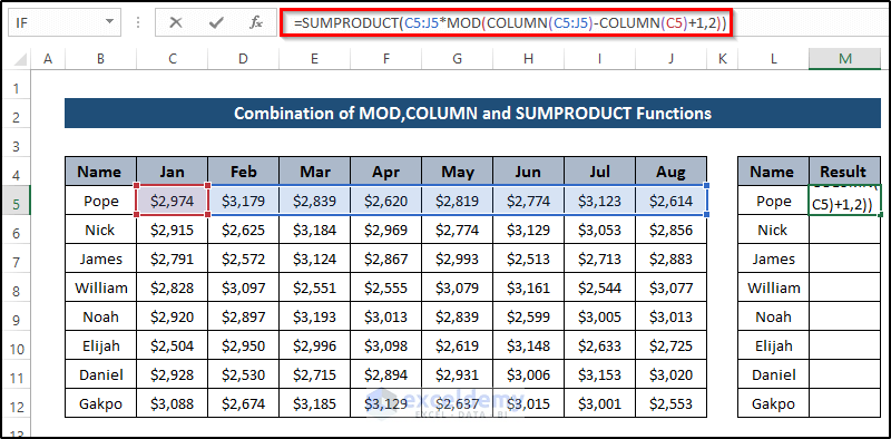
- Then, press Enter to apply the formula.
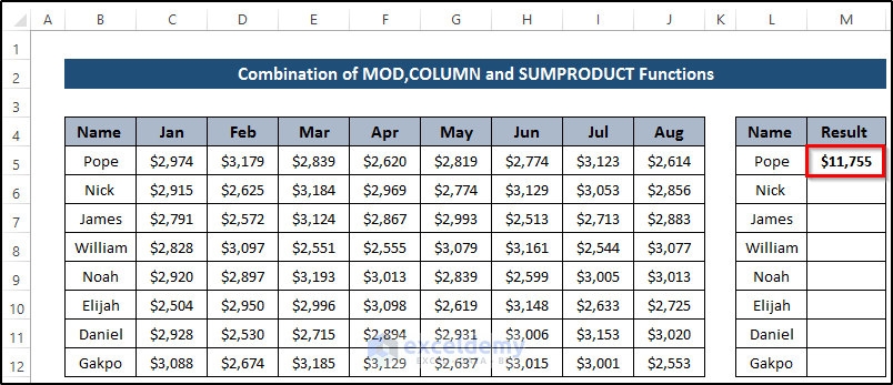
- After that, drag the Fill handle icon down the column.
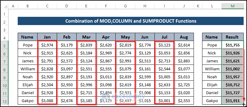
- As a result, we will get the sum of all salesman’s sales amount in several months.
- In this method, we skip column D, column F, column H, and column J. So, the summation is created using other columns.
🔎 Breakdown of the Formula
SUMPRODUCT(C5:J5*MOD(COLUMN(C5:J5)-COLUMN(C5)+1,2))
⇒ MOD(COLUMN(C5:J5)-COLUMN(C5)+1,2): Here, the COLUMN function counts the total number of columns in the given reference. Then, we subtract COLUMN(C5) and after that add 1 to the formula. This is done because if you insert a new column before the reference, it can’t change its value of it. In the formula box, click on F9 to show the output. It returns all 8 columns. Then, use the MOD function which returns a remainder after a number is divided by a divisor. We set a divisor 2. As a result, it returns (1,0,1,0,1,0,1,0). You can see it when you click on F9 on the formula box.
⇒ SUMPRODUCT(C5:J5*MOD(COLUMN(C5:J5)-COLUMN(C5)+1,2)): After that, the SUMPRODUCT function returns the sum of the given array. Here, we use the product of the range of cells C5 to J5 and the output of the MOD function. It adds the value where the MOD function value is 1 and neglects the value where the MOD function returns 0.
Read More: How to Skip a Column When Selecting in Excel
2. Applying SUM, COLUMN and IF Functions
Our next method is based on the combination of SUM, COLUMN, MOD, and IF Functions. In this method, we will put the MOD and COLUMN functions in the IF function and then, apply the IF condition there. Finally, use the SUM function of the values returned from the IF function. To understand the method, follow the steps carefully.
Steps
- First, select cell M5.
- Then, write down the following formula in the formula box.
=SUM(IF(MOD(COLUMN($C5:$J5),2)=0,$C5:$J5,0))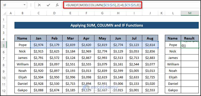
- Then, press Ctrl+Shift+Enter to apply the formula. As it is an array formula, that’s why you need to do this. In other cases, you can simply press Enter to apply the formula.
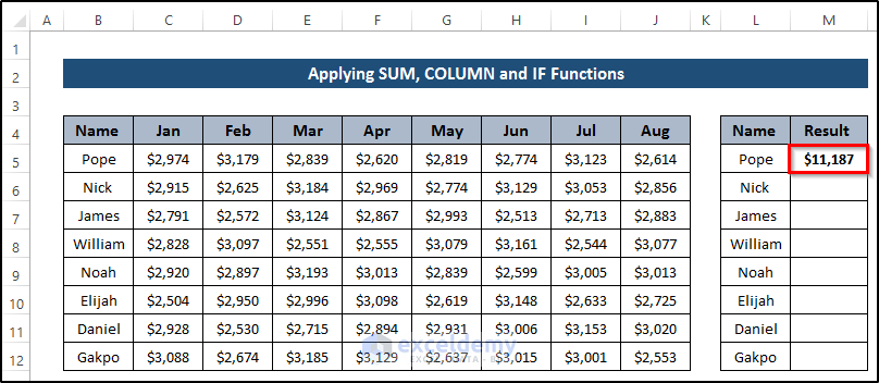
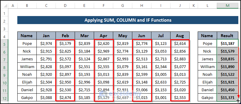
- After that, drag the Fill Handle icon down the column.
- Here, we give a condition when the MOD function returns zero, we add those columns.
- Other columns will be ignored.
- Here, we skip column C, Column E, column G, and column I. Then, add other columns using the SUM function.
🔎 Breakdown of the Formula
SUM(IF(MOD(COLUMN($C5:$J5),2)=0,$C5:$J5,0))
⇒ MOD(COLUMN($C5:$J5),2)=0: At first, the COLUMN function returns the total number of columns. In the formula box, click F9 to get the output. Using this reference, it gives (3,4,5,6,7,8,9,10).Then, it puts in the MOD function where it divides by 2. The MOD function returns a remainder after a number is divided by a divisor.
⇒IF(MOD(COLUMN($C5:$J5),2)=0,$C5:$J5,0): Then, put the previous formula of MOD and COLUMN function as a criterion of IF function. This formula denotes that if the remainder is zero then, go to the range of cells C5 to J5. Otherwise, it returns zero.
⇒ SUM(IF(MOD(COLUMN($C5:$J5),2)=0,$C5:$J5,0)): After that, the return value from the IF function will put in the SUM function. The SUM function will add all the columns which accept the condition. Finally, it returns the summation of those columns skipping other columns.
Read More: How to Skip to Next Cell If a Cell Is Blank in Excel
3. Embedding VBA Code
Our last method is based on the VBA code by Visual Basic. Here, we use a VBA code to skip other columns in the Excel formula. To understand it properly, follow the steps where we will include the code and explanation.
Steps
- First, go to the Developer tab on the ribbon.
- Then, select the Visual Basic option from the Code group.
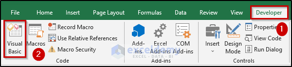
- It will open up the Visual Basic window.
- Then, go to the Insert tab at the top.
- After that, select the Module option.
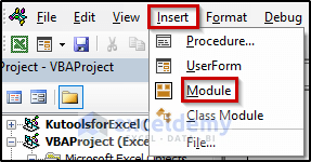
- As a result, a Module code window will appear.
- Write down the following code.
Function SumIntervalColumns(WorkRng As Range, interval As Integer) As Double
Dim ar As Variant
Dim tot As Double
tot = 0
ar = WorkRng.Value
For K = interval To UBound(ar, 2) Step interval
tot = tot + ar(1, K)
Next
SumIntervalColumns = tot
End Function- Close the Visual Basic Window.
- Then, go to cell M5.
- Write down the following formula in the formula box.
=SumIntervalColumns(C5:J5,2)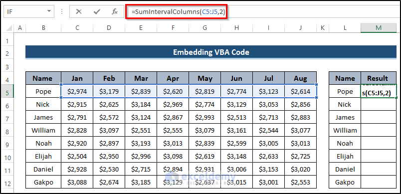
- Press Enter to apply the formula.
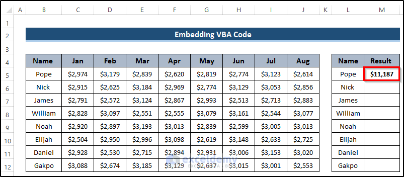
- Then, drag the Fill Handle icon down the column.
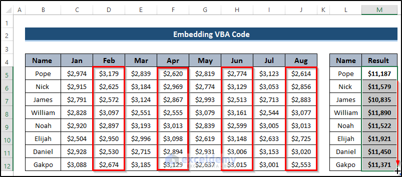
- Here, we give a condition when the MOD function returns zero, we add those columns.
- Other columns will be ignored.
- Here, we skip column C, Column E, column G, and column I. Then, add other columns using the SUM function.
🔎 VBA Code Explanation
Function SumIntervalColumns(WorkRng As Range, interval As Integer) As DoubleFirst, you need to define the function name as double.
Dim ar As Variant
Dim tot As Double
Next, declare the necessary variable for the macro.
tot = 0
ar = WorkRng.Value
After that, set tot as zero and ar as a range.value property which returns a value that represents the value of a specified range.
For K = interval To UBound(ar, 2) Step interval
tot = tot + ar(1, K)
Next
Then, take a for loop where we set an interval. Then, add the previous tot value to the present value. It continues up to the defined range.
SumIntervalColumns = totAfter that, define the function and its return value.
End FunctionFinally, end the function procedure of the macro.
Read More: How to Skip Cells in Excel Formula
Things to Remember
- In the second method, you have to press Ctrl+Shift+Enter to apply the formula. Otherwise, you don’t get results because it’s an array function.
- In the first method, you can use only MOD(COLUMN(C5:J5) instead of MOD(COLUMN(C5:J5)-COLUMN(C5)+1. But it gives a rigid solution. If you insert a new column before the range of cells, the overall solution will change. But MOD(COLUMN(C5:J5)-COLUMN(C5)+1 provides a dynamic solution.
Download Practice Workbook
Download the practice workbook below.
Conclusion
To skip every other column in the Excel formula, we have shown three methods including a VBA code and Excel functions. Hare, we discussed how to do the summation of the columns skipping every other column using the Excel formula. I think we covered all possible areas of this topic. If you have any further questions, feel free to ask in the comment section.
Related Articles
- Excel Formula to Skip Rows Based on Value
- How to Skip Hidden Cells When Pasting in Excel
- Skip Cells When Dragging in Excel
- How to Skip Blank Rows Using Formula in Excel
- How to Skip Lines in Excel
- Skip to Next Result with VLOOKUP If Blank Cell Is Present
- How to Skip Columns in Excel Formula
<< Go Back to Skip Cells | Excel Cells | Learn Excel
Get FREE Advanced Excel Exercises with Solutions!
