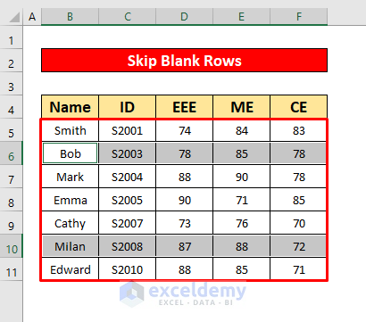
The sample dataset contains blank rows.
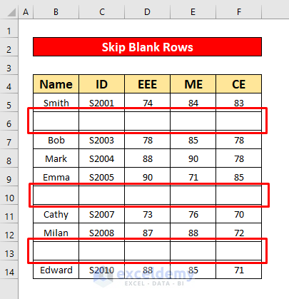
Method 1 – Using Keyboard Shortcuts to Skip Blank Rows in Excel
Step 1:
- Select B5:F14, and press F5.
- In the Go To window, enter the cell reference B5:F14 in Reference.
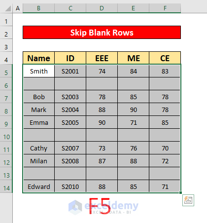
- Click Special.
![]()
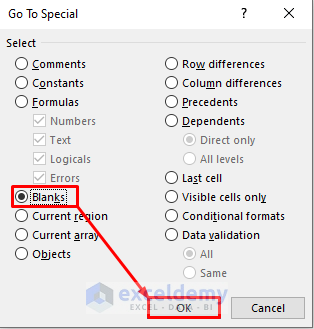
- In the Go To Special dialog box, select Blank in Select.
- Click OK.
Step 2:
You can see the blank rows.
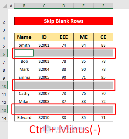
- Press Ctrl + minus(-).
- In the Delete window, select Entire row in Delete.
- Click OK.
![]()
This is the output.
Read More: How to Skip Cells in Excel Formula
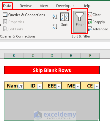
Method 2 – Using the Delete Command to Skip Blank Rows in Excel
Step 1:
- Select B4:F14.
- In the Data tab, go to:
Data → Sort & Filter → Filter
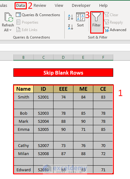
- The Filter will be enabled in the column headers.
- Click the Filter sign and check Blank.
- Click OK.
![]()
Step 2:
- In the Home tab, go to:
Home → Cells → Delete → Delete Sheet Rows
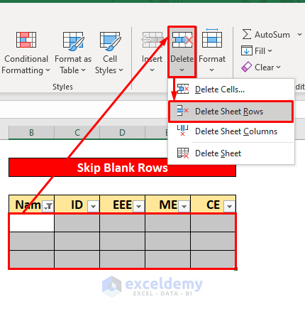
- Click Delete Sheet Rows.
- To remove the Filter sign from the header, go to:
Data → Sort & Filter → Filter
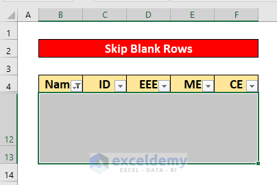
This is the output.
![]()
Read More: How to Skip Lines in Excel
Method 3 – Applying the COUNTBLANK Function to Skip Blank Rows in Excel
Step 1:
- Enter the following formula in G5.
=COUNTBLANK(B5:F5)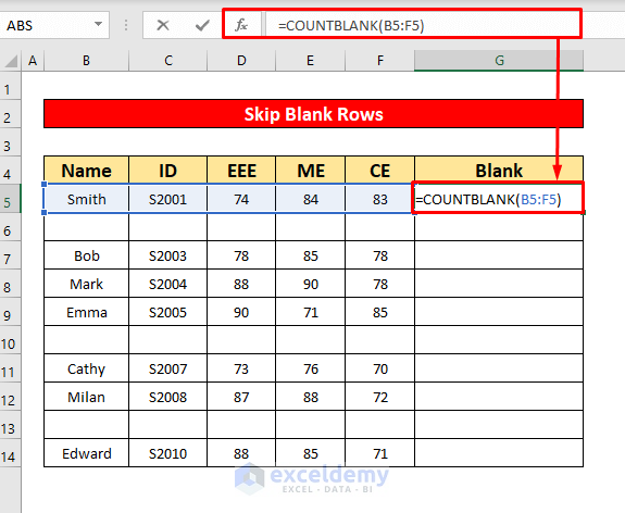
- Press ENTER.
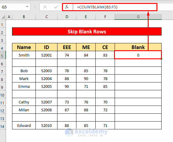
0 is returned by the COUNTBLANK function.
- Drag down the Fill Handle to see the result in the rest of the cells.
![]()
Step 2:
You can see the count of blank cells.
- Select the whole data table.
- Press CTRL + SHIFT + L to enable the Filter feature.
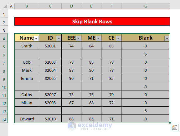
- Click the drop-down icon in the Blank column.
- Select 0 and click OK.
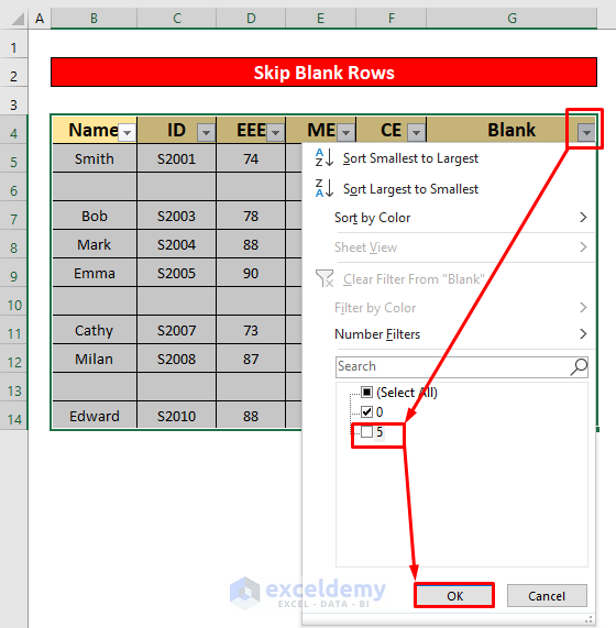
This is the output.
![]()
Read More: How to Skip Columns in Excel Formula
Method 4 – Using the FILTER Function to Skip Blank Rows in Excel
Steps:
- Enter the following formula in G5.
=FILTER(B5:E14,(B5:B14<>"")*(C5:C14<>"")*(D5:D14<>"")*(E5:E14<>""))(B5:B14<>”” ) ▶ Checks for blank cells in column B.
(C5:C14<>””) ▶ Looks for blank cells in column C.
(D5:D14<>””) ▶ Finds blank cells within column D.
(E5:E14<>””) ▶ Checks column E for blank cells.
The formula filters all blank cells, keeping the rows without blank cells only.
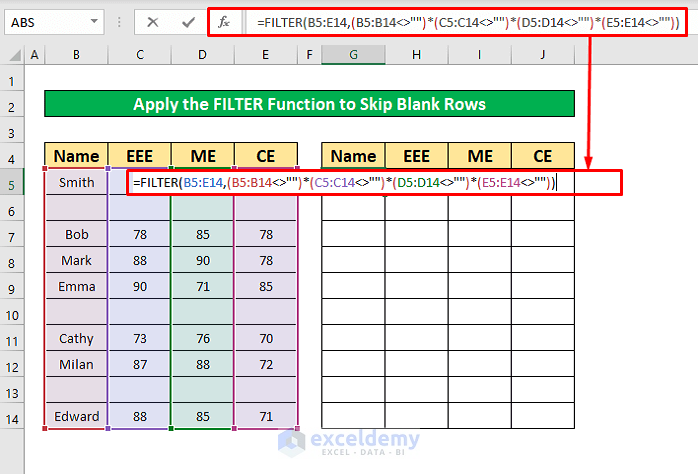
- Press ENTER.
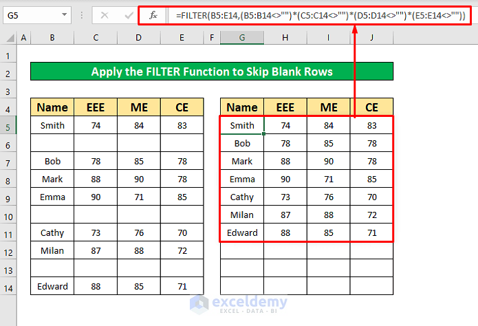
This is the output.
Read More: Excel Formula to Skip Rows Based on Value
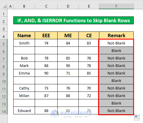
Method 5 – Merge the IF, AND & ISBLANK Functions to Skip Blank Rows in Excel
Step 1:
- Enter the following formula in F5.
=IF(AND(ISBLANK(B5), ISBLANK(C5),ISBLANK(D5),ISBLANK(E5)),"Blank", "Not-Blank")ISBLANK(B5) ▶ finds blank cells.
AND(ISBLANK(B5), ISBLANK(C5),ISBLANK(D5),ISBLANK(E5) ▶ the formula searches from column B to column E in the 5th row of the worksheet.
The whole formula finds blank rows.
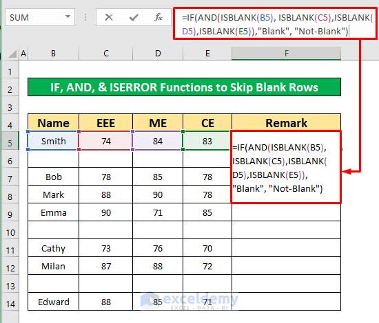
- Press ENTER.
You will see Not-Blank as the output.
![]()
- Drag down the Fill Handle to see the result in the rest of the cells.
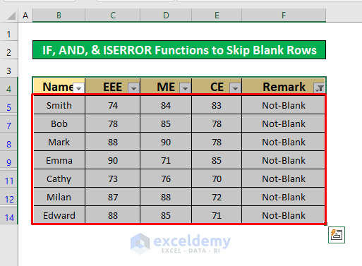
Step 2:
- Select the whole data table and press CTRL + SHIFT + L to apply the Filter feature.
- Click the drop-down icon in the Blanks column header.
- Uncheck Blank.
- Click OK.
![]()
- Press ENTER.
This is the output.
Read More: How to Skip a Column When Selecting in Excel
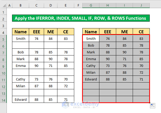
Method 6 – Combine the IFERROR, INDEX, SMALL, IF, ROW, & ROWS Functions to Skip Blank Rows
Step 1:
- Enter the following formula in G5.
=IFERROR(INDEX(B:B,SMALL(IF(B$5:B$14<>"",ROW(B$5:B$14)), ROWS(B$5:B5))), "")ROW(B$5:B$14) ▶ starts from row 5.
ROWS(B$5:B5) ▶ returns 1.
ROW(B$5:B$14)),ROWS(B$5:B5) ▶ indicates that the formula is applied to the first column of the 5th row.
SMALL(IF(C$5:C$14<>””,ROW(C$5:C$14)),ROWS(C$5:C5)) ▶ finds the smallest cell address in the 5th row.
The formula checks whether there are blank cells in the 5th row and returns the whole row if there aren’t any blank cells.
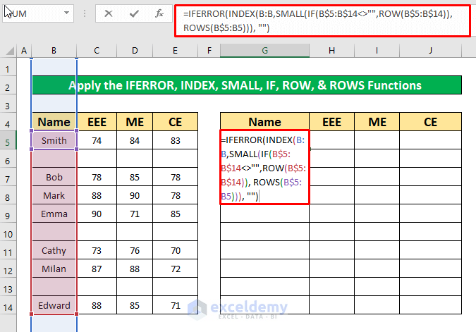
- Press ENTER.
Smith is the output.
![]()
Step 2:
- Drag the Fill Handle icon to J5.
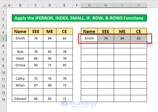
- Drag it again to cell J11.
- All rows with blank cells are excluded.
Method 7 – Merge the IF, ROWS, COUNT, INDEX, SMALL, ROW, and ROWS Functions to Skip Blank Rows in Excel
Steps:
- Enter the following formula in G5.
=IF(ROWS(B$5:B5)>COUNTA(B:B),"",INDEX(B:B,SMALL(IF(B$5:B$14<>"", ROW(B$5:B$14)),ROWS(B$5:B5))))ROW(B$5:B$14) ▶ considers rows from the 5th to the thirteenth.
ROWS(B$5:B5) ▶ indicates the first cell of the row.
INDEX(B:B,SMALL(IF(B$5:B$14<>””,ROW(B$5:B$14)),ROWS(B$5:B5))) ▶ Checks the 5th row for blank cells. As there are no blank cells in the 5th row, it returns the first element of the 5th row, which is Smith.
The formula checks for blank rows within the entire table and returns rows with no blank cells.
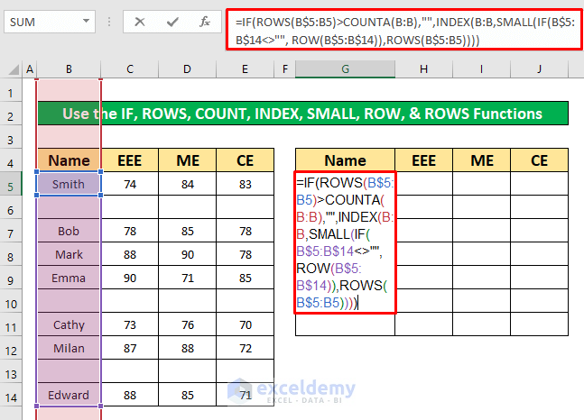
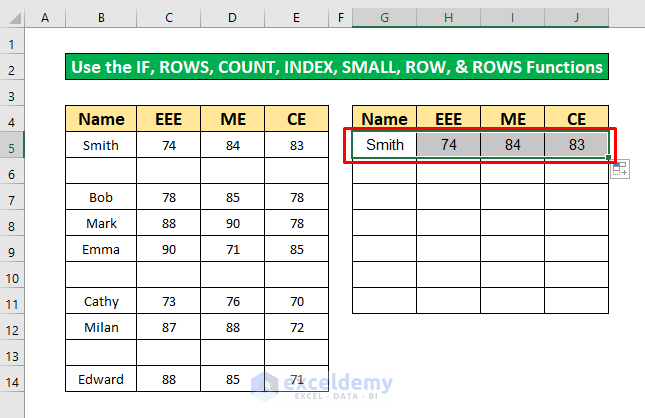
- Press ENTER.
Smith is the output.
![]()
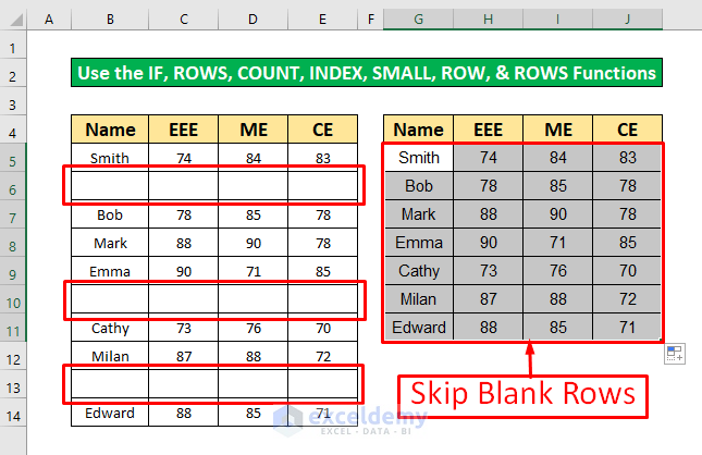
- Drag the Fill Handle to column J.
- Drag it again to the end of the CE.
This is the output.
Method 8 – Run a VBA Code to Skip Blank Rows in Excel
Step 1:
- In the Developer tab, go to:
Developer → Visual Basic
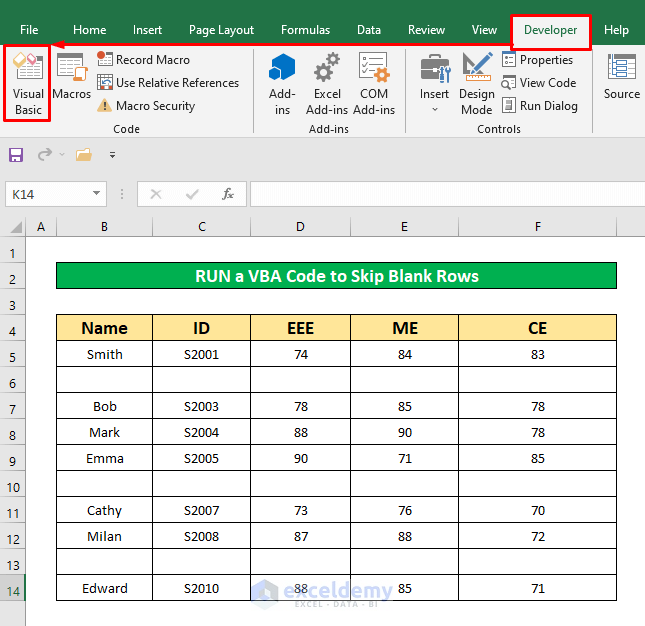
- Select Visual Basic.
- The Microsoft Visual Basic for Applications – Skip Blank Rows will be displayed.
- Go to:
Insert → Module
![]()
Step 2:
- In the Skip Blank Rows module, enter the VBA code.
Sub Skip_Blank_Rows()
Range("B5:F14").Select
Selection.SpecialCells(xlCellTypeBlanks).EntireRow.Delete
End Sub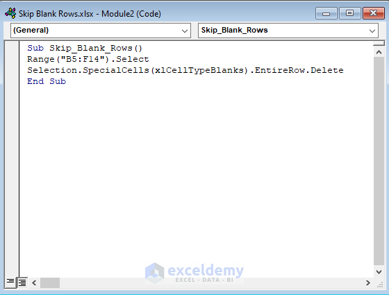
- To run the VBA:
Run → Run Sub/UserForm
![]()
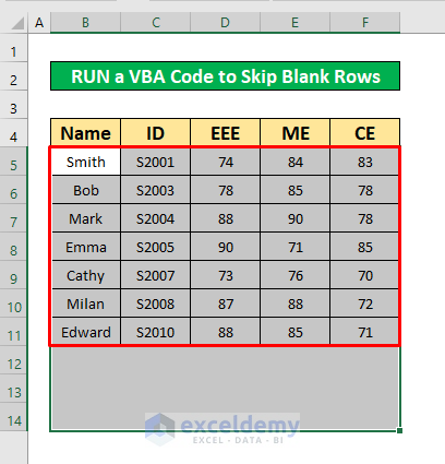
Step 3:
- Go back to the active worksheet.
This is the output.
Things to Remember
#NAME occurs when the range name is incorrect.
#REF! occurs when a cell reference is not valid.
The FILTER function is available in Excel 365 only.
Download Practice Workbook
Download the practice workbook.
Related Articles
- How to Skip Cells When Dragging in Excel
- How to Skip Hidden Cells When Pasting in Excel
- Skip to Next Result with VLOOKUP If Blank Cell Is Present
- How to Skip to Next Cell If a Cell Is Blank in Excel
<< Go Back to Excel Cells | Learn Excel
Get FREE Advanced Excel Exercises with Solutions!
