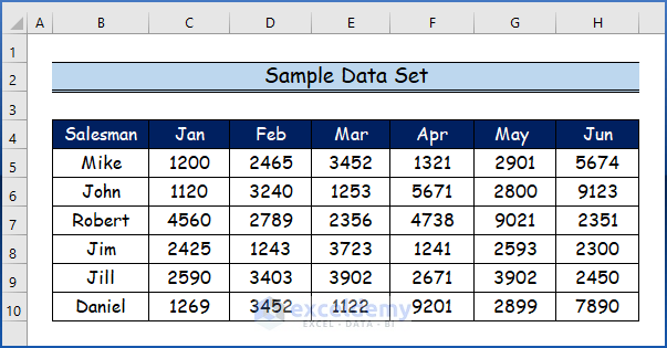
Dataset Overview
Let’s suppose we have a sample data set containing various Salesmen and their sales per month (January to June).
Method 1 – Utilizing SUMPRODUCT, MOD, and COLUMN Functions to Skip Columns
Formula Syntax:
- SUMPRODUCT: This function multiplies corresponding elements in arrays and then adds the results.
- Syntax:
=SUMPRODUCT(array1,[array2],...)-
- Arguments:
- array1: The first input array whose elements you want to multiply and then add.
- array2 (optional): The second input array whose elements you want to multiply and then add.
- Arguments:
- MOD: The MOD function calculates the remainder after dividing a number by another number.
- Syntax:
=MOD(number, divisor)-
- Arguments:
- number: The value for which you want to find the remainder.
- divisor: The number by which you want to divide.
- Arguments:
- COLUMN: The COLUMN function returns the column number of a referenced cell or range.
- Syntax:
=COLUMN(reference)-
- Arguments:
- reference: The cell or range of cells.
- Arguments:
Step-by-Step Process
Step 1:
- Select cell K5.
- Enter the following formula:
=SUMPRODUCT(C5:H5*MOD(COLUMN(C5:H5)-COLUMN(C5)+1,2))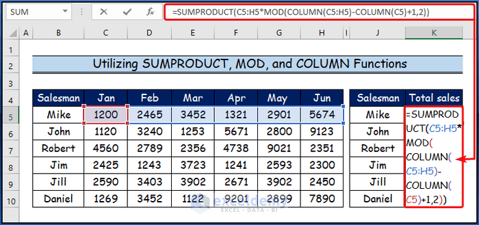
Formula Breakdown
- We use three functions: SUMPRODUCT, MOD, and COLUMN.
- MOD(COLUMN(C5:H5) – COLUMN(C5) + 1, 2):
- The COLUMN function returns the column number of the referenced range (C5:H5).
- We modify the formula by subtracting COLUMN(C5) and adding 1. This adjustment ensures that inserting a new column before the reference won’t affect the result.
- The MOD function calculates the remainder after dividing the modified column number by 2.
- SUMPRODUCT(C5:H5 * MOD(…)):
- The SUMPRODUCT function returns the total value of the resulting array.
- We combine the result of the MOD function with the range of cells C5 to H5.
- It ignores values when the MOD function gives 0 but adds them when the MOD function returns 1.
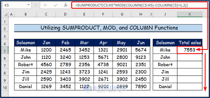
Step 2:
- Press ENTER to apply the formula.
- The K5 cell will display the total sales for the first salesman.
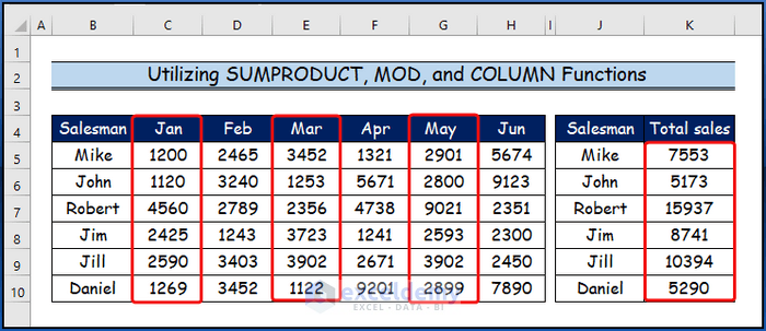
Step 3:
- Use the Fill Handle tool to drag the formula down from K5 to K10.
- You’ll get the sum of sales over several months for all salesmen.
- Columns D, F, and H are skipped in the calculation.
Read More: How to Skip a Column When Selecting in Excel
Method 2 – Incorporating SUM, COLUMN, and IF Functions to Skip Columns in Excel
Formula Syntax:
- SUM: The SUM function adds up a series of numbers.
- Syntax:
=SUM(number1,[number2],...)-
- Arguments:
- number1: The first number you want to add.
- number2 (optional): The second number you want to add.
- Arguments:
- COLUMN: The COLUMN function returns the column number of a referenced cell or range.
- Syntax:
=COLUMN(reference)-
- Arguments:
- reference: The cell or range of cells.
- Arguments:
- IF: The IF function evaluates a logical test and returns different values based on the result.
- Syntax:
=IF(logical_test, [value-if_true], [value_if_false])-
- Arguments:
- Logical_Test indicates a quantity or logical statement that can be determined to be TRUE or FALSE.
- Value_if_true demonstrates the value that will be returned if the logical test evaluates to TRUE.
- Value_if_false demonstrates the value that will be returned if the logical test evaluates to FALSE.
- Arguments:
Step-by-Step Process
Step 1:
- Select cell K5.
- Enter the following formula:
=SUM(IF(MOD(COLUMN($C5:$H5),2)=0,$C5:$H5,0)) 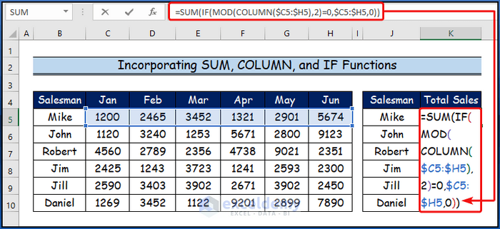
Formula Breakdown
- We’ll use three functions: SUM, COLUMN, and IF.
- MOD(COLUMN($C5:$H5), 2) = 0:
- The COLUMN function returns the column number of the referenced range ($C5:$H5).
- The MOD function calculates the remainder after dividing the modified column number by 2.
- IF(MOD(COLUMN($C5:$H5), 2) = 0, $C5:$H5, 0):
- We use the previous MOD and COLUMN functions as the criterion for the IF function.
- If the remainder is zero, it selects the cells in the range $C5:$H5; otherwise, it yields 0.
- SUM(IF(MOD(COLUMN($C5:$H5), 2) = 0, $C5:$H5, 0)):
- The SUM function adds up the values returned by the IF function.
- It includes only columns that meet the requirement (i.e., where the remainder is zero).
- Other columns are excluded from the calculation.
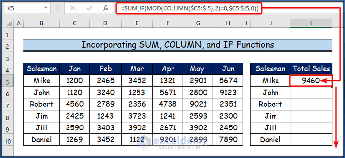
Step 2:
- Press ENTER to apply the formula.
- K5 will display the total sales for the first salesman.
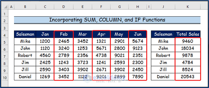
Step 3:
- Use the Fill Handle tool to drag the formula down from K5 to K10.
- You’ll get the total sales made by all salespeople over time.
- Columns C, E, and G are excluded from the calculation.
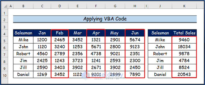
Method 3 – Applying VBA Code to Skip Columns in Excel
- Setting Up VBA:
- Open your Excel workbook.
- Press Alt + F11 to launch the VBA editor.
- In the last section, we’ll generate a VBA code that simplifies skipping columns in Excel formulas.
- Creating the Custom Function:
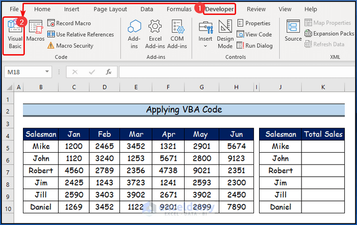
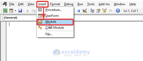
- Open the Developer tab (if not visible, enable it in Excel options).
- Click on Visual Basic to open the VBA window.
- Insert a new Module (from the Insert menu) to write the VBA code.
- VBA Code:
- Now, paste the following VBA code into the Module.
'Specifying the function name
Function SkipColumns(WorkRange As Range, interval As Integer) As Double
'Declaring variables
Dim ar As Variant
Dim x As Double
'Setting value for x and ar
x = 0
ar = WorkRange.Value
'Using For Loop
For i = interval To UBound(ar, 2) Step interval
x = x + ar(1, i)
Next
SkipColumns = x
End Function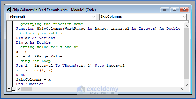
VBA Code Breakdown
- We define a function named SkipColumns that takes two arguments:
- WorkRange: The range of cells where you want to skip columns.
- interval: The interval (number of columns to skip).
- Inside the function:
- We declare variables (ar for the range values and
xfor the total). - Initialize x to zero and store the values of WorkRange in ar.
- Use a For loop to iterate through the columns based on the specified interval.
- Accumulate the values in x.
- Return the calculated value.
- We declare variables (ar for the range values and
- Using the Custom Function:
- Select cell K5.
- Enter the following formula:
=SkipColumns(C5:H5,2)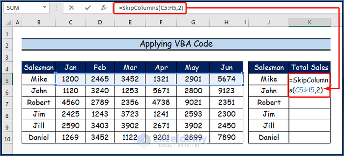
- Press ENTER to apply the formula.
- K5 will display the total sales for the first salesman.
- Drag the Fill Handle tool from K5 to calculate totals for other salesmen.
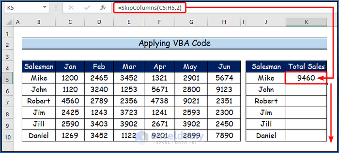
- Result:
- You’ll observe the total sales made by all salespeople over time.
- Columns C, E, and G are excluded from the calculation.
Read More: How to Skip Cells in Excel Formula
Download Practice Workbook
You can download the practice workbook from here:
Related Articles
- Excel Formula to Skip Rows Based on Value
- How to Skip Hidden Cells When Pasting in Excel
- Skip Cells When Dragging in Excel
- How to Skip Blank Rows Using Formula in Excel
- How to Skip Lines in Excel
- Skip to Next Cell If a Cell Is Blank in Excel
- Skip to Next Result with VLOOKUP If Blank Cell Is Present
<< Go Back to Excel Cells | Learn Excel
Get FREE Advanced Excel Exercises with Solutions!
