How to Skip Lines in Excel (4 Suitable Ways)

Blank lines in a Microsoft Excel spreadsheet are rather common phenomena. Most of them are redundant, and they take up additional space on the disorganized spreadsheet. As a result, users may want to skip those lines from Excel. Fortunately, Microsoft Excel provides a number of alternatives for removing blank rows from a spreadsheet. We may, however, use formulas to avoid them entirely. Today, in this post, we’ll discover practical strategies to skip blank lines/rows in Excel using formulas and other tools.

Download Practice Workbook

You can download the practice workbook from the following download button.

4 Ways to Skip Lines in Excel

You can use Excel functions, suitable Excel formulas, and other Excel tools to skip lines or rows. Let’s move forward to learn all the methods suitable for different situations.

1. Excel Formula to Skip Lines

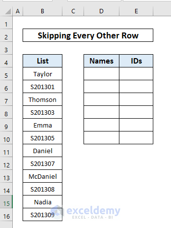
Assume we have a list of several Students and their IDs in the accompanying rows. We wish to segregate them into two columns. As a result, we will skip such rows utilizing various methods.

In this part of the article, we will see the following cases.

1.1 Skip Every Other Row

We will use a formula that is a combination of Excel INDEX and ROWS functions. Apply the following simple steps.

Steps:

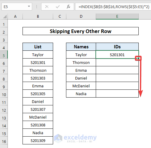
• First and foremost, we’ve added two new columns called Names and IDs. We intend to divide the List into those two columns.

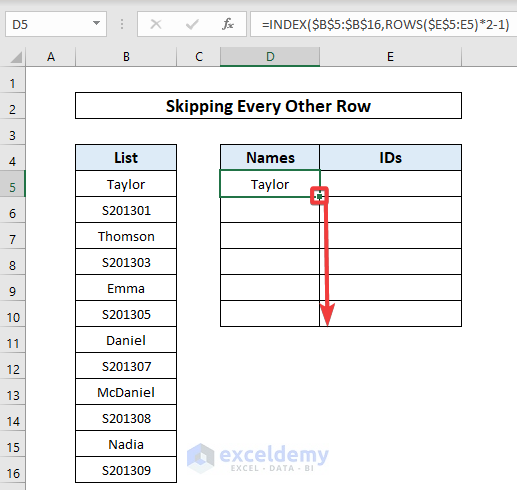
• In cell D5, enter the following formula:

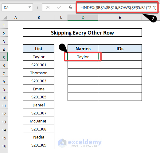
• We’ll now drag the Fill handle down to fill the following cells with the same formula.

• In cell E5, enter the following formula:

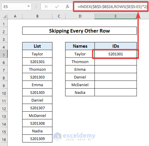
• For this time, we’ll drag the fill handle down to fill the following cells with the same formula.

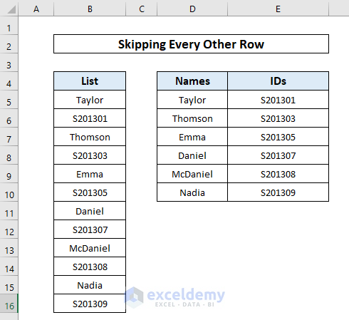
• So, this is how the final range will appear.

An Alternative Way to Skip Every Other Row:

You can also use MOD and ROW functions, then apply the Filter command to Skip Even or Odd Rows.

Steps:

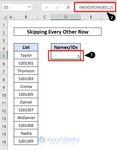
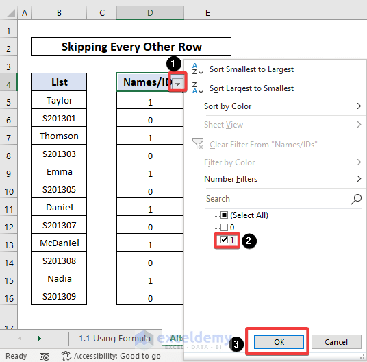
• Enter the formula=MOD(ROW(B5),2)in Cell D5 in a blank cell. Take a look at the image below:

• Now drag down the fill handle.
• Select the D4 cell and press the Filter icon under the Data tab.

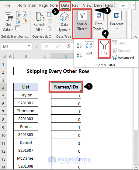
• In Cell D4, click the Arrow, uncheck (Select All), and select 1 in the filter box. Look at the image below:

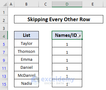
• Here is the final image with the names only. We can copy those names for further purposes.

1.2 Skip Every N-th Row

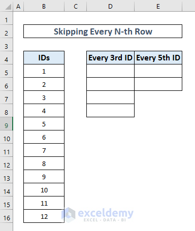
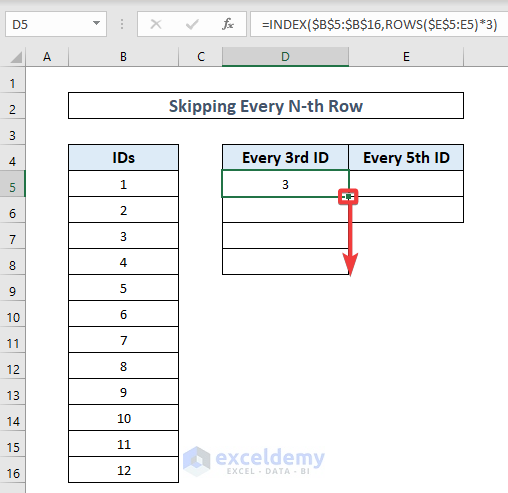
Assume we have a list of many IDs in the rows below. But we want to divide them into two columns to distinguish Every 3rd ID and Every 5th ID. As a result, we will skip such rows using the methods listed below.

Now, execute the following steps to perform our desired task.

Steps:

• In cell D5, enter the following formula:

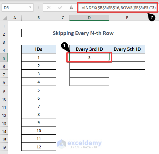
• This time, we’ll drag the fill handle down to fill the subsequent cells with the same formula.

• In cell E5, enter the following formula:

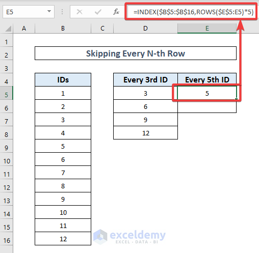
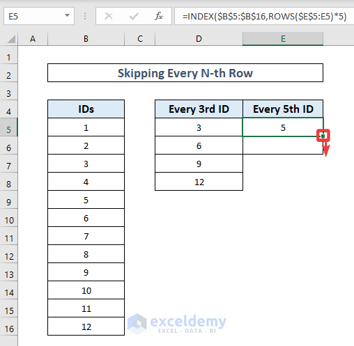
• Now, drag the fill handle icon to fill the next cells with the formula.

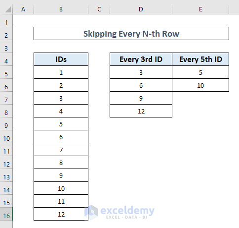
• So, this is how the final range will appear.

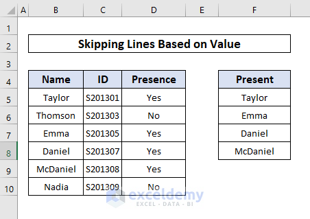
1.3 Skip Lines Based on Value

Imagine we have a long list of names, IDs, and their Presence. However, we need the names of present pupils in a separate column. As a result, we will use the methods given below to skip such rows that include “No”.

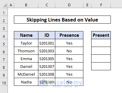
Steps:

• In cell D5, enter the following formula:

• Now, we’ll drag the fill handle down to fill the following cells with the same formula.

• As a consequence, this is how the final range will be.

Read More: Excel Formula to Skip Rows Based on Value (7 Examples)

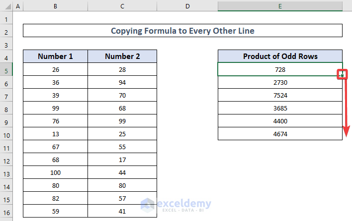
2. Skip Every Other Line While Copying Formula

Assume we have a list of numbers 1 and 2. However, we require the product of Numbers 1 and 2 in odd rows. As a consequence, we will skip even rows using the methods listed below.

Steps:

• In cell E5, enter the following formula:

• Now, we’ll drag the fill handle down to fill the following cells with the same formula and get the product of odd rows.

Read More: How to Skip Cells in Excel Formula (8 Easy Methods)

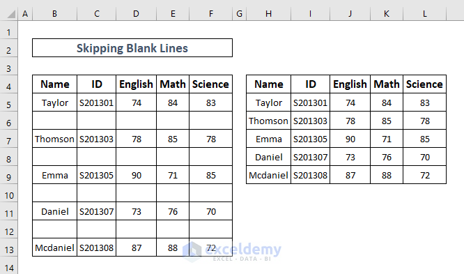
3. Skip Blank Rows with FILTER Function

To easily filter out all the blank rows from an Excel spreadsheet, we will utilize the FILTER function. This function uses a dynamic array. That is, if you simply run this function in one cell, it will automatically cover all the associated cells where the formula result should be. Now, follow the procedures below to do this.

Steps:

• In cell H5, enter the following formula:

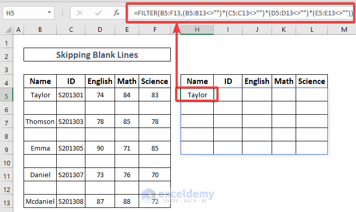
• So, this is how the final range will be.

Read More: Skip to Next Result with VLOOKUP If Blank Cell Is Present

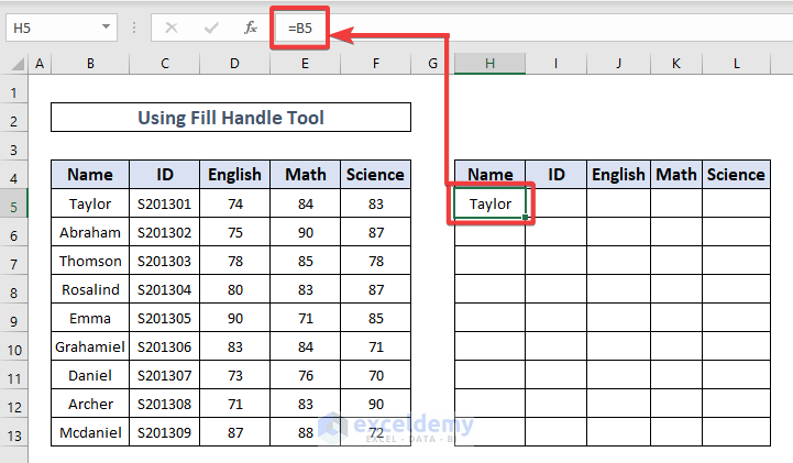
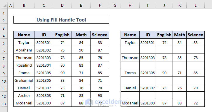
4. Skip Lines with Fill Handle Tool

Whenever dealing with data in Excel, users may see duplicate or undesired rows after each important row. There are several methods for copying every other row to a separate region while duplicating only the essential data.

Steps:

• Type a formula =B5 in H5 that refers to the first cell in the range to be copied in a blank cell to the right of the rows to duplicate.

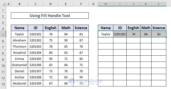
• All the information from the first row of the range is displayed after dragging the fill handle across the columns.

• As seen in the illustration, highlight the first row as well as the blank row just beneath it. Drag down with the mouse on the fill handle to autofill the range.

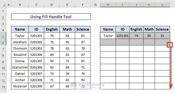
• So, this is the final range that we required.

Read More: How to Skip to Next Cell If a Cell Is Blank in Excel (5 Easy Ways)

Conclusion

From time to time, users may need to eliminate empty rows from spreadsheets. Fortunately, Microsoft Excel gives a variety of choices, as seen in the preceding approaches. Feel free to follow those instructions and download the workbook to use for your own practice. Please visit ExcelDemy and post any questions, problems, or recommendations in the comments box.

Related Articles

• How to Skip Hidden Cells When Pasting in Excel (2 Methods)
• Skip Cells When Dragging in Excel (4 Easy Methods)
• How to Skip Columns in Excel Formula (3 Easy Ways)
• Skip Every Other Column Using Excel Formula (3 Methods)
• How to Skip a Column When Selecting in Excel (4 Easy Methods)