How to Skip to Next Cell If a Cell Is Blank in Excel (5 Easy Ways)

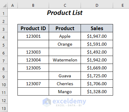
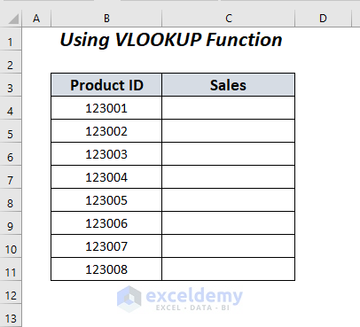
Consider the following dataset containing a list of Ids, Products, and their corresponding Sales values. In the Product ID column and Product column, we have some blank cells. Using some formulas, we will skip these blank cells and retrieve values from the adjacent cells.

We used the Microsoft Excel 365 version in this article, but you can use any other version at your disposal.

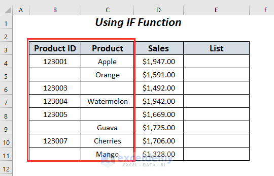
Method 1 – Using IF Function

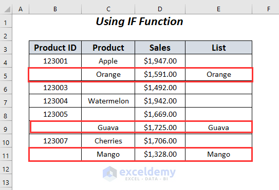
Let’s use the IF function to make a list of products which don’t have corresponding Product IDs. When there is no value in a cell in the Product ID column, we’ll move to the adjacent cell and extract the value into the List column.

Steps:

• Enter the following formula in cell E4:

Here, B4 is the Product ID, and C4 is the corresponding Product name. If cell B4 is blank, the formula returns the product name Apple, otherwise a blank.

• Press ENTER and drag down the Fill Handle to return the values for the rest of the column.

The following results are returned in the List column.

Read More: How to Skip Blank Rows Using Formula in Excel

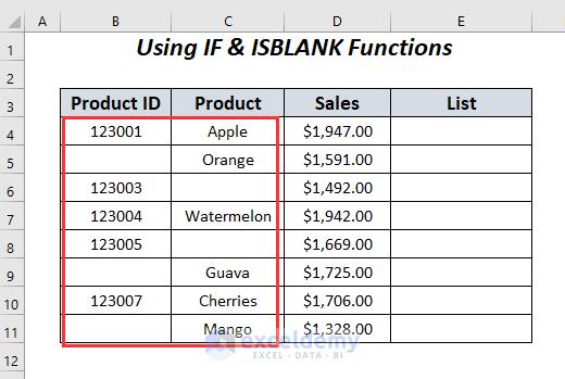
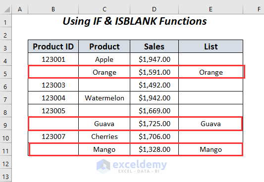
Method 2 – Using IF and ISBLANK Functions

Here, we will extract the names of the products which don’t have corresponding Product IDs into the List column using a combination of the IF and ISBLANK functions.

Steps:

• Enter the following formula in cell E4:

Here, B4 is the Product ID, and C4 is the corresponding Product name. If cell B4 is blank, then the formula returns the product name Apple, otherwise a blank.

• Press ENTER and drag down the Fill Handle.

A list of names of products without ids is returned.

Read More: How to Skip a Column When Selecting in Excel

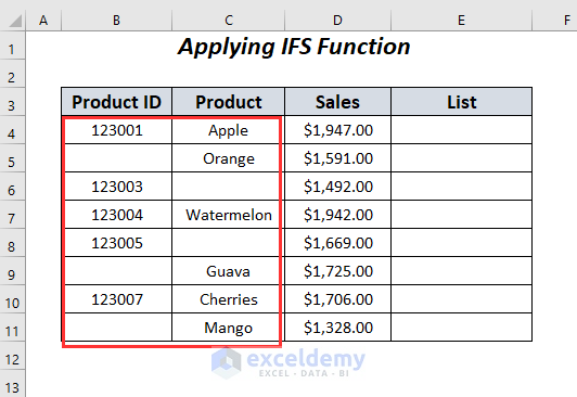
Method 3 – Using the IFS Function

Here, we will skip the blank cells in the Product ID column and move to the adjacent cell in the Product column to extract the name of the products, then gather them in the List column using the IF, ISNA, and IFS functions.

Steps:

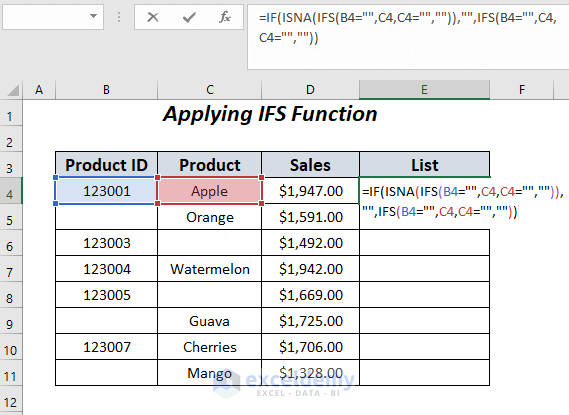
• Enter the following formula in cell E4:

Here, B4 is the Product ID, and C4 is the corresponding Product name.

• Press ENTER and drag down the Fill Handle.

A list of products without Product Ids is returned in the List column.

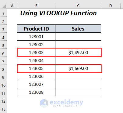
Method 4 – Using a Combination of IFERROR, VLOOKUP and IF Functions

Here, we will search for the sales values in the Sales column, and then using the IFERROR, VLOOKUP and IF functions, we will skip the blank cells of the Product column and move to the Sales column to extract the corresponding sales values.

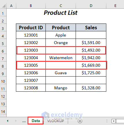
We will extract the values from the Sales column into the following datasheet in a new sheet.

Steps:

• Enter the following formula in cell C4:

Here, B4 is the Product ID.

• Press ENTER and drag down the Fill Handle.

The sales values for the blank products are returned in the Sales column of the new sheet.

Read More: Skip to Next Result with VLOOKUP If Blank Cell Is Present

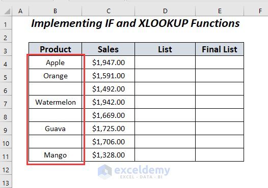
Method 5 – Using the IF and XLOOKUP Functions

Now we’ll apply the combination of the IF and XLOOKUP functions to return the name of the product just above a blank cell in the Product column in the List column. Then we will filter these values using the FILTER function.

Steps:

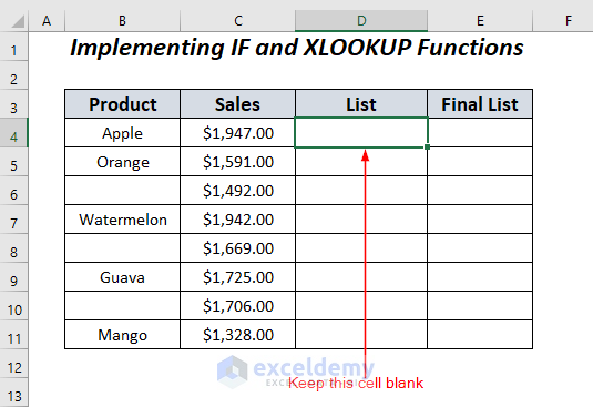
• Keep the initial cell of the List column Blank.

• Enter the following formula in cell D5:

=IF(B5=””,IF(B5=””,XLOOKUP(“*”,$B$4:B5,$B$4:B5,””,2,-1),””),IF(B5<>””,””,IF(D4=””,””,B5)))

• Press ENTER and drag down the Fill Handle.

The result is as follows:

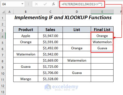
In cell E4, use the following formula to remove the blanks from the List column:

Here, D4:D11 is the range in which we will be filtering out the blanks.

Read More: How to Skip Columns in Excel Formula

Download Practice Workbook

Related Articles

• Excel Formula to Skip Rows Based on Value
• How to Skip Hidden Cells When Pasting in Excel 
• Skip Cells When Dragging in Excel
• How to Skip Cells in Excel Formula
• How to Skip Lines in Excel

<< Go Back to Excel Cells | Learn Excel