How to Skip Cells in Excel Formula (8 Easy Methods)

This tutorial will demonstrate how to skip cells in an Excel formula. When dealing with lots of data, sometimes we have to skip unnecessary cells for ease of work. Moreover, after using certain if it’s not needed anymore, then it should be easily skipped to avoid confusion. So, it is very to learn how to skip cells in an Excel formula.


How to Skip Cells in Excel Formula: 8 Easy Methods

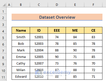
We’ll use a sample dataset overview as an example in Excel to understand easily. In this case, we have the Name in column B, ID in column C, EEE, ME, and CE in columns D, E, and F. If you follow the steps correctly, you should learn how to skip cells in the Excel formula on your own. The steps are:

how to skip cells in excel formula


1. Use of Filter Option

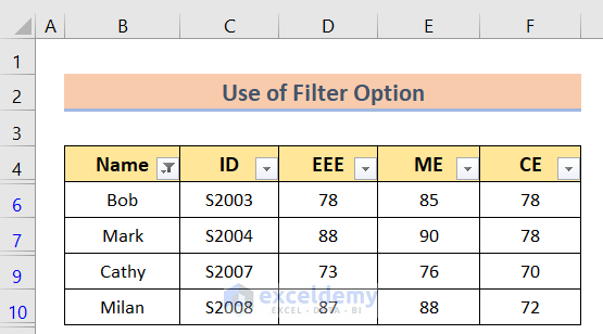
Now, we want to skip cells by using the Filter Option. This is the easiest way to skip cells in Excel. The steps of this method are as follows.

Steps:

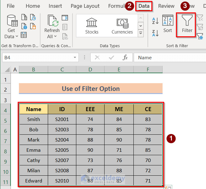
  • At first, go to select the table > Data > Filter options.

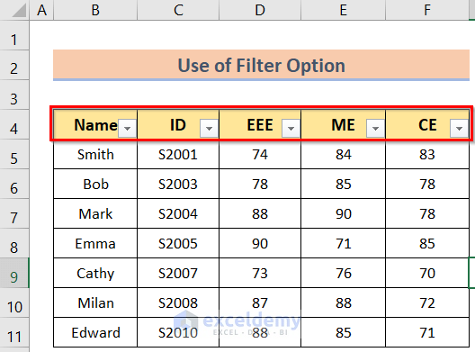
  • Second, you will get the result like the below image.

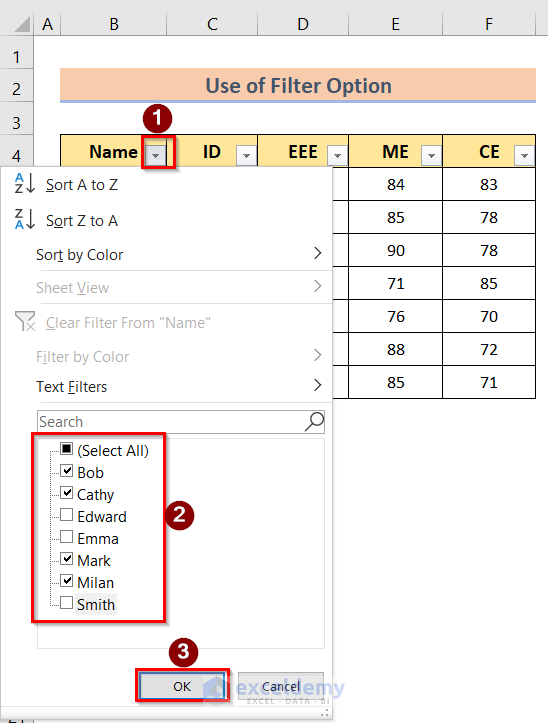
  • Third, click on the filter point (in this case Name), untick the desired data, and press OK.

Using the Text Filters to Skip Cells in Excel Formula

  • Last, you will get the desired result.

Read More: How to Skip Hidden Cells When Pasting in Excel


2. Utilizing COUNTBLANK Function

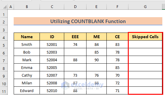
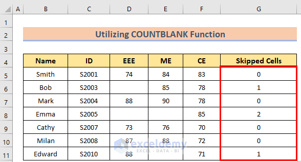
Next, we can skip cells by using the COUNTBLANK function. This function is used for counting. In our case, we will use this function to count skip cells. We can learn the method by following the below steps.

Steps:

  • To begin with, create a dataset similar to the below image.

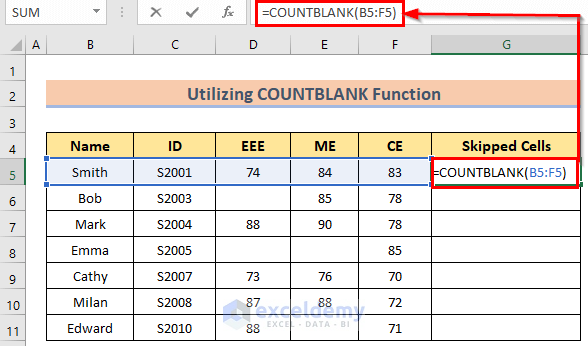
  • In addition, insert the following formula in cell G5.
=COUNTBLANK(B5:F5)

Inserting COUNTBLANK Function to Skip Cells in Excel Formula

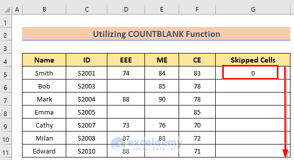
  • Furthermore, you will get results for the cell.
  • Then, use the Fill Handle to apply it to all desired cells.

  • Next, you will get the desired result.

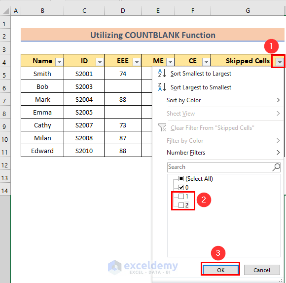
  • After that, go to select the table > Data > Filter options like the first method. Then click on the filter point, untick the desired cells, and press OK.

Using the Text Filters to Skip Cells in Excel Formula

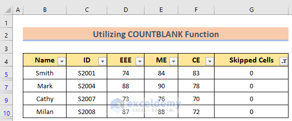
  • Finally, you will get the desired result.

Read More: How to Skip to Next Cell If a Cell Is Blank in Excel


3. Applying FILTER Function

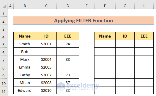
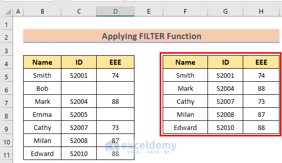
In this case, we aim to skip cells by applying the FILTER function. The work of this function is to filter a data range and give a filtered result. To learn this method, we have to follow the below steps.

Steps:

  • Firstly, create a dataset like the below image.

  • Secondly, insert the following formula in cell F5.
=FILTER(B5:D11,(B5:B11<>"")*(C5:C11<>"")*(D5:D11<>""))
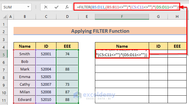
Inserting Filter Function to Skip Cells in Excel Formula

  • Lastly, after pressing the Enter button, you will get the desired result.

Read More: Skip Cells When Dragging in Excel


4. Combining IF, AND & ISBLANK Functions

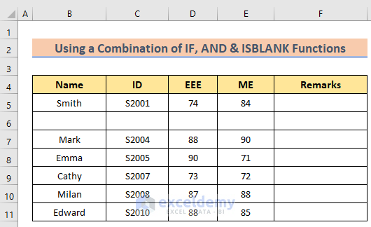
We can also apply a combination of IF, AND & ISBLANK functions to skip cells. The If function gives logical comparison, and the And function returns if the condition is true or false, but when the cell has no information but still true or false comparison is needed then the ISBLANK function is used.  The steps of this method are.

Steps:

  • First, arrange a dataset like the below image.

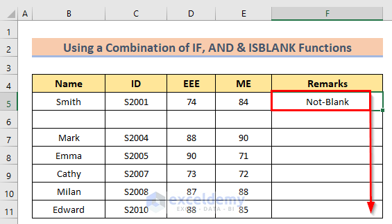
  • Next, insert the following formula in cell F5.
=IF(AND(ISBLANK(B5), ISBLANK(C5),ISBLANK(D5),ISBLANK(E5)),"Blank", "Not-Blank")
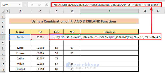
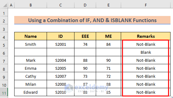
Using combination of IF, AND & ISBLANK Functions to Skip Cells in Excel Formula

  • After that, you will get the result for the cell and then use the Fill Handle option.

  • Afterward, you will get the below result.

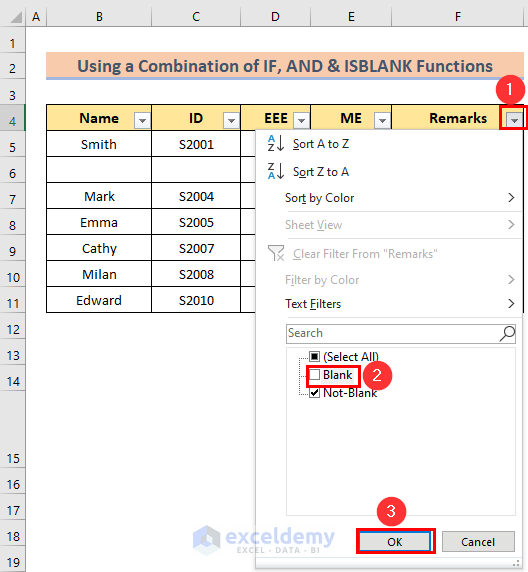
  • Next to that, go to select the table > Data > Filter options like the first method. Then click on the filter point, untick the desired cells, and press OK.

Using the Text Filters to Skip Cells in Excel Formula

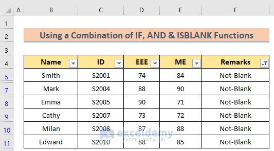
  • Finally, after pressing the Enter button, you will get the desired result.

🔎 How Does the Formula Work?

  • ISBLANK(E5)): It represents the selected cell E5.
  • AND(ISBLANK(B5), ISBLANK(C5), ISBLANK(D5), ISBLANK(E5)), “Blank”, “Not-Blank”: This portion presents the selected cell the conditions will be applied on.
  • IF(AND(ISBLANK(B5), ISBLANK(C5),ISBLANK(D5),ISBLANK(E5)),”Blank”, “Not-Blank”): This portion presents the condition in the function.

Read More: Skip to Next Result with VLOOKUP If Blank Cell Is Present


5. Combining IFERROR, INDEX, SMALL, IF, ROW & ROWS Functions

Now, we will combine multiple functions to skip cells. The IFERROR function traps and handles errors in a formula, the INDEX function returns a value within a range, the SMALL function categorizes Excel data statistically and the ROW or ROWS functions are mainly used in counting selected rows or numbers. We have to follow the below steps to learn this whole method.

Steps:

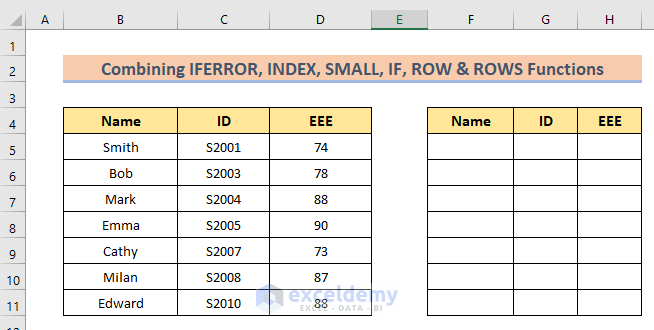
  • First, arrange a dataset like the below image.

  • Second, insert the following formula in cell F5.
=IFERROR(INDEX(B:B,SMALL(IF(B$5:B$11<>"",ROW(B$5:B$11)), ROWS(B$5:B5))), "")
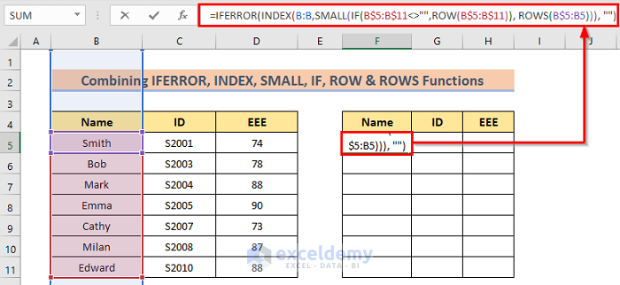
Inserting combinition of IFERROR, INDEX, SMALL, IF, ROW & ROWS Functions to Skip Cells in Excel Formula

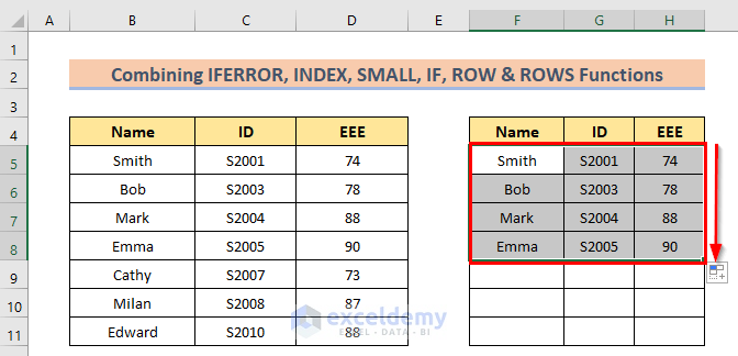
  • Last, after pressing the Enter button, you will get the desired result.

🔎 How Does the Formula Work?

  • ROWS(B$5:B5): This portion represents the reference cell.
  • ROW(B$5:B$11): this portion represents the selected range of the cell.
  • SMALL(IF(B$5:B$11<>””,ROW(B$5:B$11)), ROWS(B$5:B5): this portion represents fixed cells of reference of columns.
  • IFERROR(INDEX(B:B,SMALL(IF(B$5:B$11<>””,ROW(B$5:B$11)), ROWS(B$5:B5))), “”): this portion presents the whole condition.

Read More: How to Skip Lines in Excel


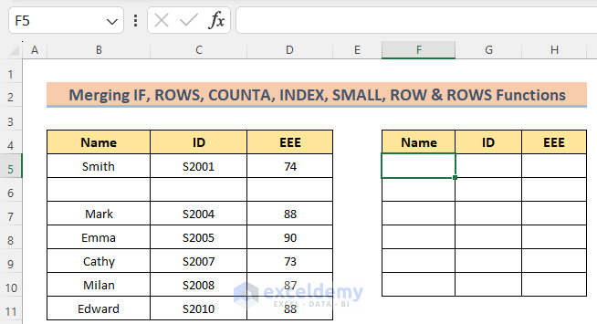
6. Merging IF, ROWS, COUNTA, INDEX, SMALL, ROW & ROWS Functions

In this case, our goal is to skip by using a combination of functions. The COUNTA function is used when a large number of data entries are needed within a certain range. All the other functions are already explained in the previous methods. The steps of this method are as follows.

Steps:

  • To begin with, arrange a dataset like the below image.

How to Skip blank cells

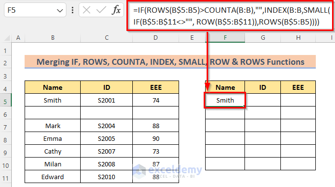
  • In addition, insert the following formula in cell F5.
=IF(ROWS(B$5:B5)>COUNTA(B:B),"",INDEX(B:B,SMALL(IF(B$5:B$11<>"", ROW(B$5:B$11)),ROWS(B$5:B5))))
  • Furthermore, after pressing the Enter button, you will get the desired result.

Merging IF, ROWS, COUNTA, INDEX, SMALL, ROW & ROWS Functions

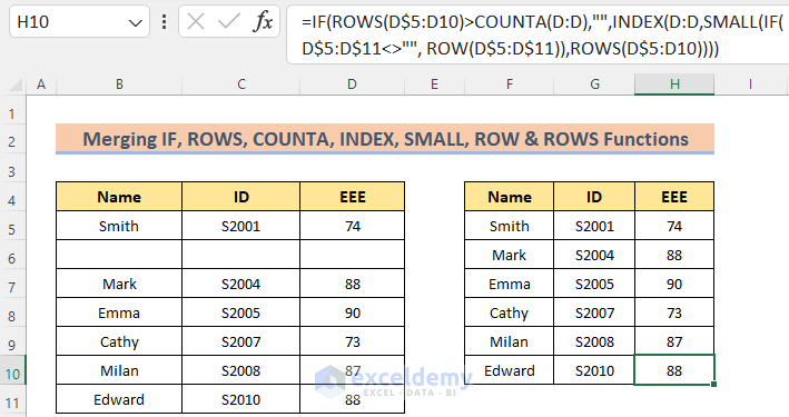
  • Finally, use the Fill Handle to get the desired result.

Skipping Balnk Cells in Excel

🔎 How Does the Formula Work?

  • ROWS(B$5:B5): This portion represents the reference cell.
  • ROW(B$5:B$11): this portion represents the selected range of the cell.
  • INDEX(B:B,SMALL(IF(B$5:B$11<>””, ROW(B$5:B$11)),ROWS(B$5:B5))): this portion represents the counta function the formula will work on.
  • IF(ROWS(B$5:B5)>COUNTA(B:B),””,INDEX(B:B,SMALL(IF(B$5:B$11<>””, ROW(B$5:B$11)),ROWS(B$5:B5)))): This portion represents the whole condition.

Read More: How to Skip Blank Rows Using Formula in Excel


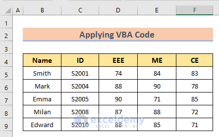
7. Applying VBA Code

We can skip cells by using the VBA code. We have to follow the below steps to learn this whole method.

Steps:

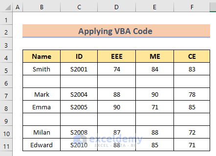
  • Firstly, arrange the dataset like the below image.

  • Secondly, press Alt+F11 options to open the VBA window.

Sub Skip_Blank_Rows()
Range("B5:F11").Select
Selection.SpecialCells(xlCellTypeBlanks).EntireRow.Delete
End Sub
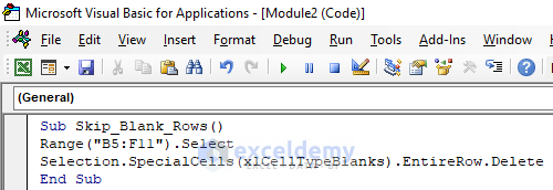
Inserting VBA code to Skip Cells in Excel Formula

  • Lastly, after pressing the RUN or F5 button, you will get the desired result.


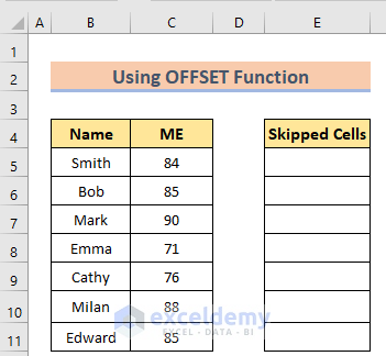
8. Using OFFSET Function

In this case, our goal is to skip cells in Excel by using the OFFSET function. When any complicated conditional result is needed, then it is the most useful method to use. The steps of this method are.

Steps:

  • First, arrange a dataset like the below image.

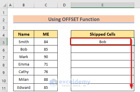
  • Next, insert the following formula in cell E5.
<span style="font-size: 14pt;">=OFFSET($B$5,ROW(D1)*2-1,0)</span>
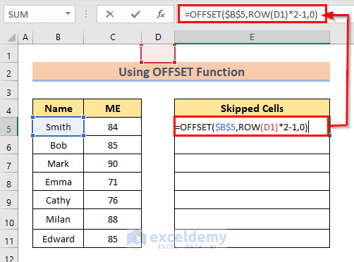
Inserting OFFSET function to Skip Cells in Excel Formula

  • After that, after pressing the Enter button, you will get the desired result.

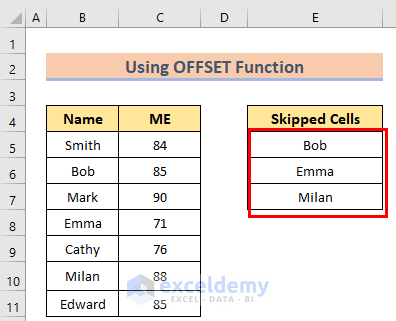
  • Finally, use the Fill Handle to get the final result.


Things to Remember

  • If there remains any error in any formula, excel will show an error.
  • The Filter Function is only available for Microsoft 365 users.
  • While using the formulas, you should give proper attention to the cell you are using. Otherwise, the formula won’t give the desired result.

Download Practice Workbook

You can download the practice workbook from here.


Conclusion

Henceforth, follow the above-described methods. Hopefully, these methods will help you to skip cells in an Excel formula. We will be glad to know if you can execute the task in any other way. Please feel free to add comments, suggestions, or questions in the section below if you have any confusion or face any problems. We will try our level best to solve the problem or work with your suggestions.


Related Articles


<< Go Back to Skip Cells  | Excel Cells | Learn Excel

Get FREE Advanced Excel Exercises with Solutions!
Zehad Rian Jim
Zehad Rian Jim

Zehad Rian Jim is a dedicated professional with a BSc. Degree in Naval Architecture and Marine Engineering from Bangladesh University of Engineering and Technology. He's good with Microsoft Office and has written more than 80 helpful articles for ExcelDemy in the last year. Now, he makes fun and easy-to-follow Excel tutorials for YouTube as part of the ExcelDemy Video project. Zehad loves figuring out Excel problems, and his passion for learning new things in Excel shines through in... Read Full Bio

We will be happy to hear your thoughts

Leave a reply

Advanced Excel Exercises with Solutions PDF


ExcelDemy
Logo