Example 1 – Using the FILTER Function
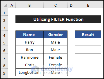
In the first example, we are going to use the FILTER function to skip rows based on value using the Excel formula. For that, we consider a dataset that has the name and gender of five employees of a company. Our dataset is in the range of cells B5:C9, and we will show our result in column E.
- Select cell E5.
- Enter the following formula. This formula will skip rows where the gender of the employees is Female:
=FILTER(B5:B9,C5:C9="Male")
- Press Enter.
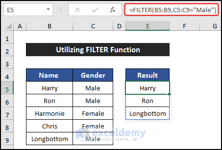
- You’ll see that the two rows with female employees are skipped, and the names of the other three employees appear in column E.
Read More: How to Skip Cells in Excel Formula
Example 2 – Applying the OFFSET Function
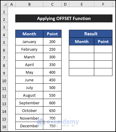
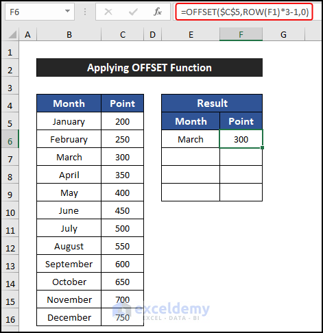
In this example, we will use the OFFSET function to skip rows based on value using the Excel formula. To demonstrate the example, we consider a dataset of 12 months with gradually increased points, and we will show our result in columns E and F. We want to get the rows after every two rows.
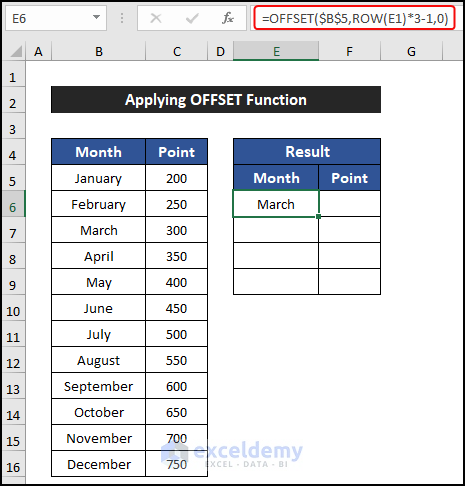
- Select cell E6.
- Enter the following formula to get the name of the months:
=OFFSET($B$5,ROW(E1)*3-1,0)
- Press Enter.
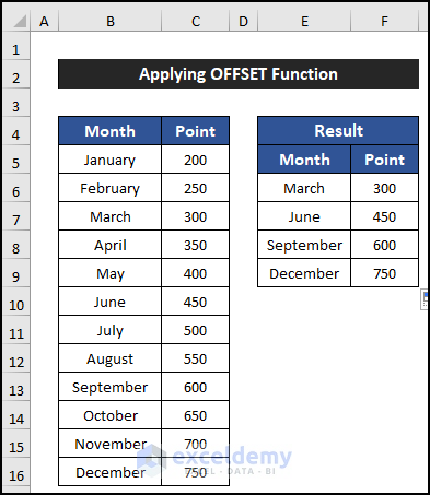
- Select cell F6 and enter this formula to get the corresponding points:
=OFFSET($C$5,ROW(F1)*3-1,0)
- Press Enter.
- Drag the Fill Handle icon from E6:F6 to copy the formulas up to cell F9.
- You’ll notice that four rows are copied, and the other two rows in between are skipped.
Read More: How to Skip Columns in Excel Formula
Example 3 – Using the INDEX and ROW Functions
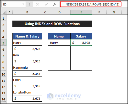
In the following example, we are going to use the INDEX and ROWS functions to skip rows based on value. Our dataset is in the range of cells B5:B14. We will skip each row after the employee’s name and show our result in column D. We will follow the same steps to obtain the salary.
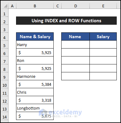
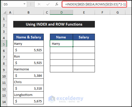
- Select cell D5.
- Enter the following formula to get the name of the employees:
=INDEX($B$5:$B$14,ROWS($E$5:E5)*2-1)
- Press Enter.
- Select cell E5 and enter this formula to get the salary of that employee:
=INDEX($B$5:$B$14,ROWS($E$5:E5)*2)
- Press Enter.
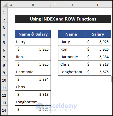
- Select the range of cells D5:E5 and drag the Fill Handle icon to copy the formulas up to cell F7.
- You’ll see that all the names and salaries are displayed in a column, with every row in between skipped.
Breakdown of the Formula (for cell D5)
- ROWS($E$5:E5): The ROWS function returns the row number. In this case, it returns 1.
- INDEX($B$5:$B$14, ROWS($E$5:E5)*2-1): The INDEX function uses the result of the ROWS function to retrieve the value from the specified row range. In this example, the value is Harry.
Read More: How to Skip Cells When Dragging in Excel
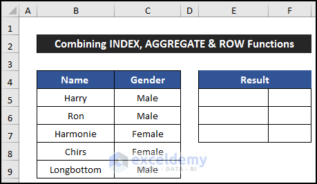
Example 4 – Combining INDEX, AGGREGATE and ROW Functions
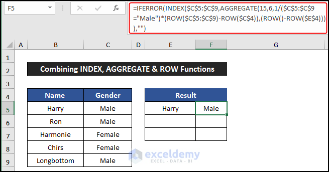
The IFERROR, INDEX, AGGREGATE, and ROW functions will help us to skip rows based on value using the Excel formula. For that, we consider a dataset that has the names and genders of five employees of a company. Our dataset is in the range of cells B5:C9, and we will show our result in columns E and F.
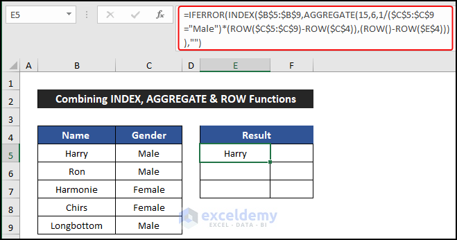
- Select cell E5.
- Enter the following formula to get the name of the employees:
=IFERROR(INDEX($B$5:$B$9,AGGREGATE(15,6,1/($C$5:$C$9="Male")*(ROW($C$5:$C$9)-ROW($C$4)),(ROW()-ROW($E$4)))),"")
- Press Enter.
- Select cell F5 and enter the following formula to get the gender of that employee.
=IFERROR(INDEX($C$5:$C$9,AGGREGATE(15,6,1/($C$5:$C$9="Male")*(ROW($C$5:$C$9)-ROW($C$4)),(ROW()-ROW($E$4)))),"")
- Press Enter.
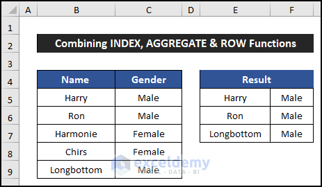
- Drag the Fill Handle icon from E5:F5 to copy the formulas up to cell F7.
- You’ll get the names and salaries of male employees, with female employees’ rows skipped.
Breakdown of the Formula (for cell E5)
- ROW($E$4): Shows the row number of cell E4 (value is 4).
- ROW(): Returns the row number of the current cell (row number is 5).
- ROW($C$4): Displays the row number of cell C4 (value is 4).
- ROW($C$5:$C$9): Provides the row numbers for cells C5 to C9.
- AGGREGATE(15, 6, 1/($C$5:$C$9=”Male”)*(ROW($C$5:$C$9)-ROW($C$4)), (ROW()-ROW($E$4))): Using values from the ROW function, AGGREGATE determines which rows to display. For this cell, the value is 1.
- INDEX($B$5:$B$9, AGGREGATE(15, 6, 1/($C$5:$C$9=”Male”)*(ROW($C$5:$C$9)-ROW($C$4)), (ROW()-ROW($E$4)))): INDEX retrieves the value based on the AGGREGATE result. Here, it returns Harry.
- IFERROR(INDEX($B$5:$B$9, AGGREGATE(15, 6, 1/($C$5:$C$9=”Male”)*(ROW($C$5:$C$9)-ROW($C$4)), (ROW()-ROW($E$4)))), “”): IFERROR checks the INDEX result. If valid, it shows the value; otherwise, it returns a blank.
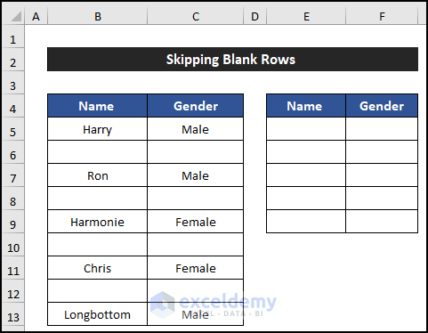
Example 5 – Skip Blank Rows
In this example, we will skip the blank rows using a formula. The FILTER function will assist in skipping the blank rows. Our dataset is in the range of cells B5:C13, and there are four blank rows. We will show our results in columns E and F.
- Select cell E5.
- Enter the following formula to skip blank rows:
=FILTER(B5:C13,(B5:B13<>"")*(C5:C13<>""))
- Press Enter.
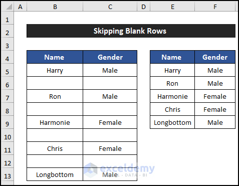
- You’ll see that all blank rows are skipped, and only rows with values are displayed in columns E and F.
Read More: How to Skip to Next Cell If a Cell Is Blank in Excel
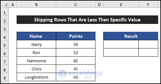
Example 6 – Skip Rows That Are Less Than a Specific Value
In this example, we will skip rows that have a value less than our desired value. The IFERROR, INDEX, AGGREGATE, and ROW functions will help us. We consider a dataset that has the names and points of five employees of a company. Our dataset is in the range of cells B5:C9, and we will show our result in columns E and F.
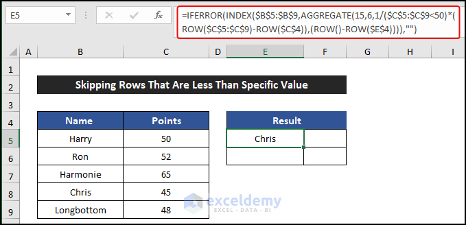
- Select cell E5.
- Enter the following formula to get the names of the employees with less than 50 points:
=IFERROR(INDEX($B$5:$B$9,AGGREGATE(15,6,1/($C$5:$C$9<50)*(ROW($C$5:$C$9)-ROW($C$4)),(ROW()-ROW($E$4)))),"")
- Press Enter.
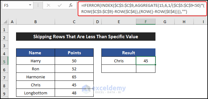
- Select cell F5 and enter this formula to get the points of those employees:
=IFERROR(INDEX($C$5:$C$9,AGGREGATE(15,6,1/($C$5:$C$9<50)*(ROW($C$5:$C$9)-ROW($C$4)),(ROW()-ROW($E$4)))),"")
- Press Enter.
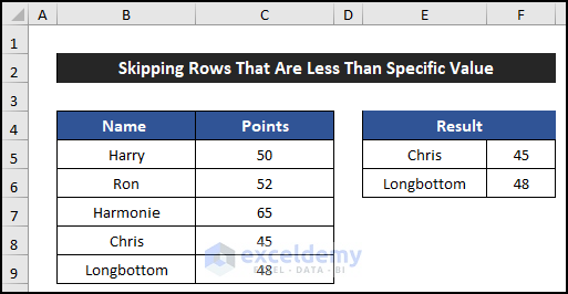
- Select the range of cells E5:F5 and drag the Fill Handle icon to copy the formulas up to cell F7.
- You’ll see the names of employees whose points are less than 50 displayed in the desired location.
Breakdown of the Formula (for cell E5)
- ROW($E$4) returns the row number of cell E4, which is 4.
- ROW() returns the row number of the current cell (E5), which is 5.
- ROW($C$4) returns the row number of cell C4, which is 4.
- ROW($C$5:$C$9) provides the row numbers for cells C5 to C9.
- AGGREGATE(15,6,1/($C$5:$C$9<50)*(ROW($C$5:$C$9)-ROW($C$4)),(ROW()-ROW($E$4))) determines which row’s value to display. In this case, it’s row 4.
- INDEX($B$5:$B$9,AGGREGATE(15,6,1/($C$5:$C$9<50)*(ROW($C$5:$C$9)-ROW($C$4)),(ROW()-ROW($E$4))) retrieves the value from column B corresponding to row 4, which is Chris.
- IFERROR(…,””) ensures that if there’s an error (e.g., no valid value), it returns a blank cell.
Example 7 – Skip Rows That Are Greater Than a Specific Value
In our last example, we are going to use the IFERROR, INDEX, AGGREGATE, and ROW functions to skip rows where the values are greater than a specific value. We consider a dataset that has the names and points of five employees of a company. Our dataset is in the range of cells B5:C9, and we will show our result in columns E and F.
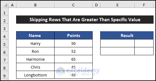
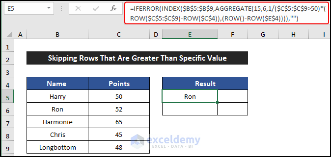
- Select cell E5.
- Enter the following formula to get the names of the employees with more than 50 points:
=IFERROR(INDEX($B$5:$B$9,AGGREGATE(15,6,1/($C$5:$C$9>50)*(ROW($C$5:$C$9)-ROW($C$4)),(ROW()-ROW($E$4)))),"")
- Press Enter.
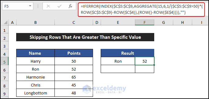
- Select cell F5 and enter this formula to get the points of those employees:
=IFERROR(INDEX($C$5:$C$9,AGGREGATE(15,6,1/($C$5:$C$9="Male")*(ROW($C$5:$C$9)-ROW($C$4)),(ROW()-ROW($E$4)))),"")
- Press Enter.
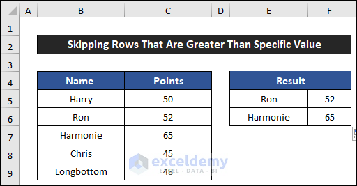
- Select the range of cells E5:F5 and drag the Fill Handle icon to copy the formulas up to cell F6.
- You’ll see the names of employees whose points are greater than 50 displayed in the desired location.
Breakdown of the Formula (for cell E5)
- ROW($E$4): The function shows the row number of cell E4. Here, the value is 4.
- ROW(): The function returns the row number of this cell. The row number is 5.
- ROW($C$4): The ROW function shows the row number of cell C4. Here, the value is 4.
- ROW($C$5:$C$9): Here, the function provides us with the row number of the cells C5 to C9.
- AGGREGATE(15,6,1/($C$5:$C$9>50)*(ROW($C$5:$C$9)-ROW($C$4)),(ROW()-ROW($E$4))): Using all the values from the ROW function the AGGREGATE function returns which rows value have to show. For this cell, the value will be 2.
- INDEX($B$5:$B$9,AGGREGATE(15,6,1/($C$5:$C$9>50)*(ROW($C$5:$C$9)-ROW($C$4)),(ROW()-ROW($E$4))): The INDEX function will use the result of the AGGREGATE function and display the value of the cell. Here, the value returns Ron.
- The IFERROR(…,””): The IFERROR function checks the result of the INDEX function. If the INDEX function returns any valid value the function will show it. Otherwise, the function will return a blank. Here, the function returns Ron.
Read More: Skip to Next Result with VLOOKUP If Blank Cell Is Present
Download Practice Workbook
You can download the practice workbook from here:
Related Articles
- How to Skip Hidden Cells When Pasting in Excel
- How to Skip a Column When Selecting in Excel
- How to Skip Lines in Excel
<< Go Back to Excel Cells | Learn Excel
Get FREE Advanced Excel Exercises with Solutions!
