Method 1 – Combine OFFSET and ROW Functions to Skip Cells When Dragging
Steps:
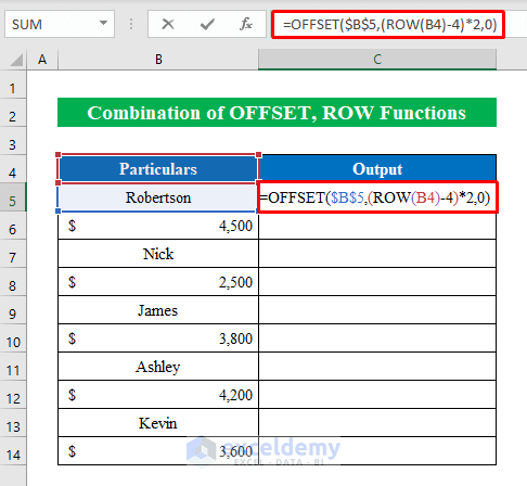
- Choose a cell to apply the formula. We selected cell (C5).
- Write the formula down-
=OFFSET($B$5,(ROW(B4)-4)*2,0)- (ROW(B4)-4) → In here the ROW function returns the row number 4. Thus the output stands (4-4) = “0”
- =OFFSET($B$5,(ROW(B4)-4)*2,0)→ The OFFSET function returns output based on a cell reference ($B$5), and then (2,0) commanding 2 rows down and 0 stands for staying in the same column.
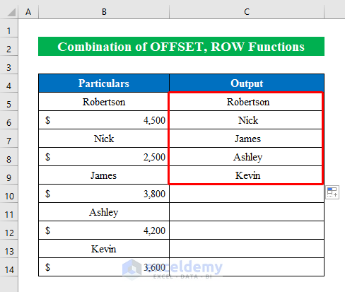
- The Enter button and drag down the “fill handle” to fill all the cells.
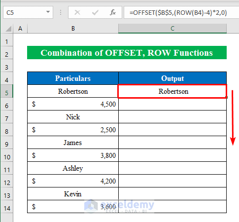
- Get the names in a new column by dragging and skipping their sales volume from the previous column.
Method 2 – Merge INDEX and ROWS Functions to Skip Cells When Dragging
Steps:
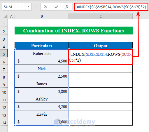
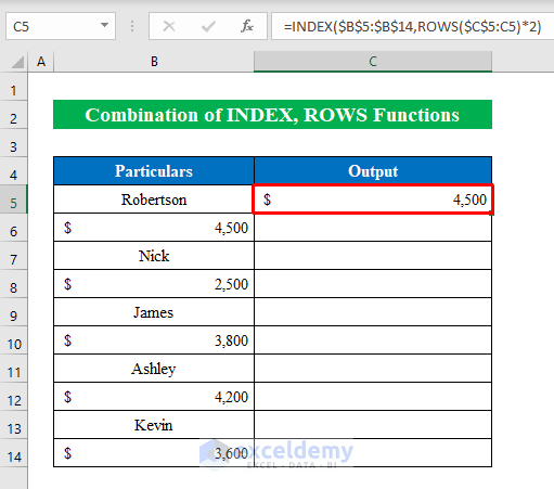
- Select a cell (C5) to apply the formula-
=INDEX($B$5:$B$14,ROWS($C$5:C5)*2)- ROWS($C$5:C5)→ Here the ROWS function extracts the row number, which provides an output -”1”
- =INDEX($B$5:$B$14,ROWS($C$5:C5)*2)→ In this part, ($B$5:$B$14) it’s the cell reference for the index function where the “ROWS($C$5:C5)*2” is the row_num extracting the data from the cell (B6) which is- “4500”.
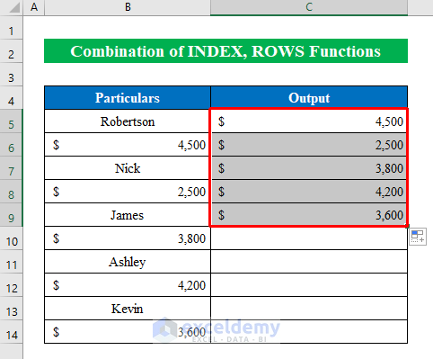
- Press Enter and pull the “fill handle” down.
- We extracted only the sales volume while skipping the cells with names when dragging.
Method 3 – Use Fill Handle to Skip Cells When Dragging in Excel
Steps:
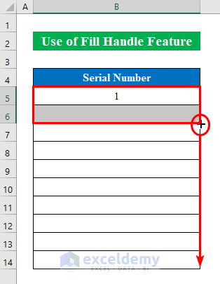
- Choose cells (B5:B6). After choosing two cells with one blank and one with the number “1” Excel automatically understands how you want to fill your cells by dragging the fill handle.
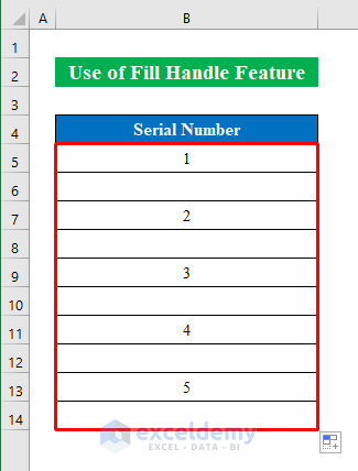
- Selecting cells pull the “fill handle” down.
- Get the output in your hands just the way you wanted, skipping cells when dragging the fill handle.
Method 4 – Combine IF, MOD, ROW, INDEX, and INT Functions to Skip Cells When Dragging
Steps:
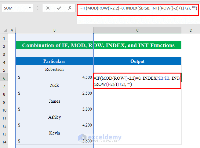
- Choose a cell to write the formula as we are extracting only the numbers from the column thus we choose cell (C6).
- Put the formula down-
=IF(MOD(ROW()-2,2)=0, INDEX($B:$B, INT((ROW()-2)/1)+2), "")
Formula Breakdown:
- (ROW()-2)→ Here the ROW function extracts the row number which is “6” as the chosen cell is cell (C6). after that subtracting with “-2”.
- Output is “4”
- INT((ROW()-2)/1)→ The INT function returns the integer number which is “4”.
- MOD(ROW()-2,2)→ The MOD function extracts the remaining from the arguments. As there are no remainings thus the output stands to “0”.
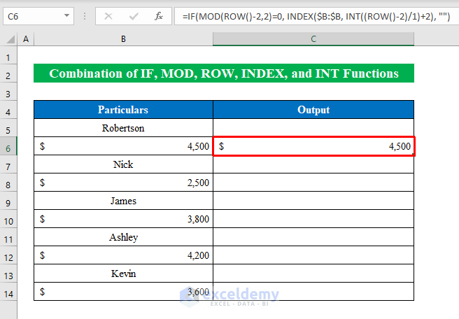
- =IF(MOD(ROW()-2,2)=0, INDEX($B:$B, INT((ROW()-2)/1)+2), “”)→ in this final part the IF function runs inside the string where after completing logical_test which is “(MOD(ROW()-2,2)=0” it goes for the argument where “INDEX($B:$B, INT((ROW()-2)/1)+2)” returns an output “4500” and if the argument is not met –” “ it will return a blank cell.
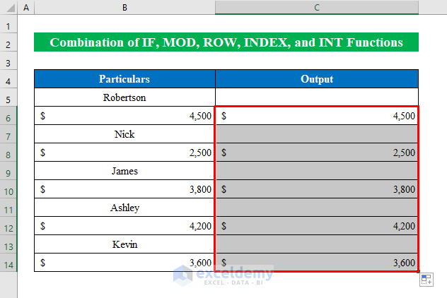
- Hit the Enter button and drag down the “fill handle”.
- The final output in our hands extracts only the sales volume. In this, we skipped cells (B5:B7:B9:B11:B13) while dragging in excel.
Things to Remember
- While applying formulas don’t forget to complete formulas with closing brackets. Otherwise, the formulas won’t work.
Download Practice Workbook
Download this practice workbook to exercise while you are reading this article.
Related Articles
- Excel Formula to Skip Rows Based on Value
- How to Skip a Column When Selecting in Excel
- How to Skip Cells in Excel Formula
- How to Skip Blank Rows Using Formula in Excel
- How to Skip Lines in Excel
<< Go Back to Excel Cells | Learn Excel
Get FREE Advanced Excel Exercises with Solutions!
