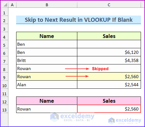
This is the sample dataset.
Method 1- Combining the VLOOKUP and the IFNA Functions
Steps:
- Enter “Ben” in B13.
- Enter the following formula in C13.
=IFNA(VLOOKUP(B13,B5:C10,2,1),VLOOKUP(B13,B5:C10,2,0))
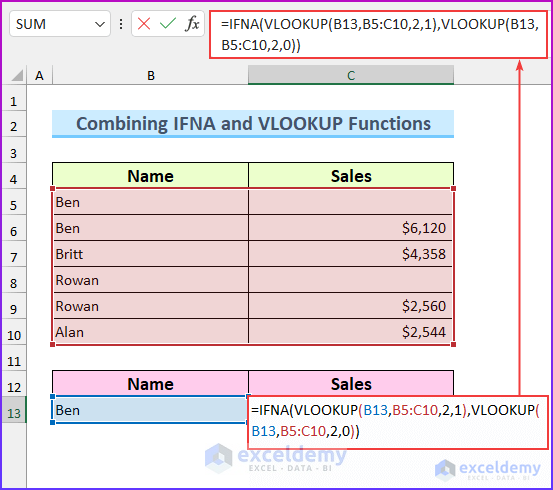
- Press ENTER.
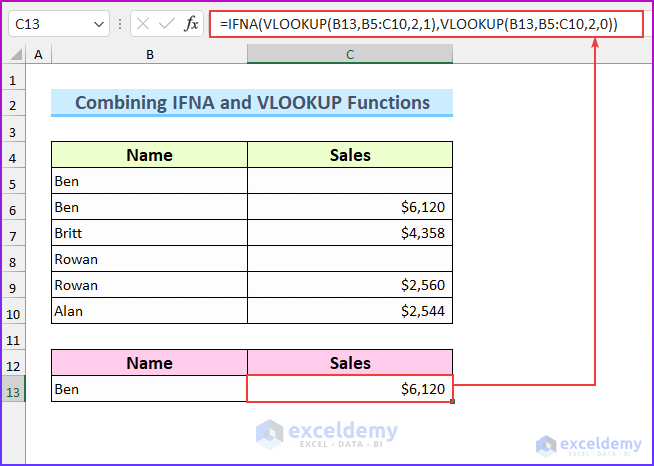
This is the output.
Formula Breakdown
- There are two VLOOKUP functions inside the IFNA function.
- VLOOKUP(B13,B5:C10,2,1)
- Output: 6120.
- matches the value in B13 with B5:C10. It returns the value from the second column. The range_lookup is set as an approximate match by typing 1.
- VLOOKUP(B13,B5:C10,2,0)
- Output: 0.
- matches the value in B13 with B5:C10. It returns the value from the second column. The range_lookup is set as an exact match by typing 0.
- The formula reduces to → IFNA(6120,0)
- Output: 6120.
- If “#N/A” is returned by the first VLOOKUP function, you will get the second value from this function.
Method 2 – Combining the IFS and VLOOKUP Functions to Skip to the Next Result
Steps:
- Enter the following formula in C13.
=IFS(VLOOKUP(B13,B5:C10,2,0)<>0,VLOOKUP(B13,B5:C10,2,0),VLOOKUP(B13,B6:C10,2,0)<>0,VLOOKUP(B13,B6:C10,2,0),VLOOKUP(B13,B7:C10,2,0)<>0,VLOOKUP(B13,B7:C10,2,0),VLOOKUP(B13,B8:C10,2,0)<>0,VLOOKUP(B13,B8:C10,2,0),VLOOKUP(B13,B9:C10,2,0)<>0,VLOOKUP(B13,B9:C10,2,0),VLOOKUP(B13,B10:C10,2,0)<>0,VLOOKUP(B13,B10:C10,2,0))
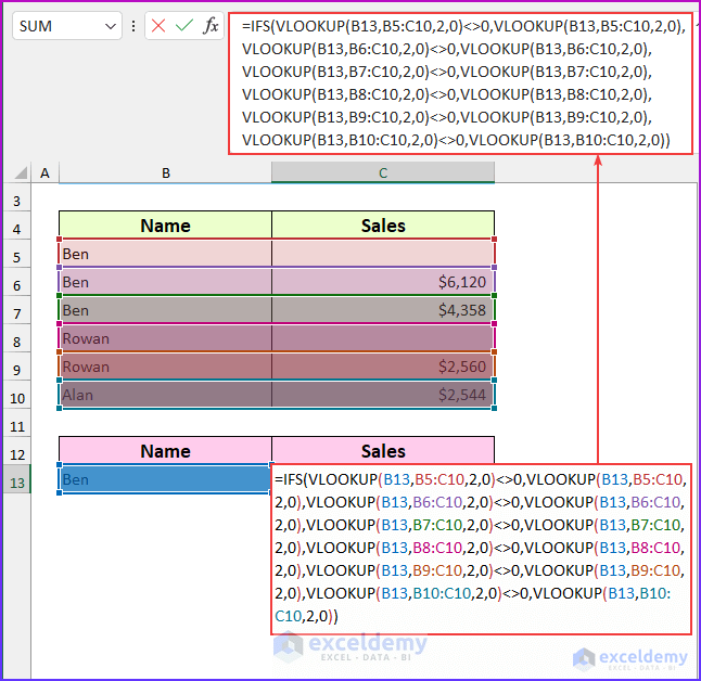
- Press ENTER.
This is the output.
![]()
Formula Breakdown
- The IFS function allows more simple formulas than the nested IF statement.
- VLOOKUP(B13,B5:C10,2,0)<>0
- Output: FALSE.
- This logical_test checks if the VLOOKUP function returns a value other than zero.
- Then, the formula searches values other than zero within a smaller range, B6:C10, B7:C10 and so on.
- Reduces to → IFS(FALSE,0,FALSE,0,FALSE,0,FALSE,0,TRUE,2560,#N/A,#N/A)
- Output: 2560.
- There is only one true value.
![]()
Read More: How to Skip Columns in Excel Formula
Method 3 – Skipping to the Next Result by Merging the IF and the VLOOKUP Functions
Steps:
- Enter the following formula in C13.
=IF(VLOOKUP(B13,B5:D10,2,0)="",VLOOKUP(B13,B5:D10,3,0),VLOOKUP(B13,B5:D10,2,0))
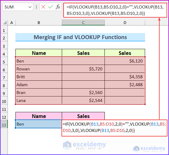
- Press ENTER.
- The formula will move to the next column, if the previous column is blank.
![]()
Read More: How to Skip to Next Cell If a Cell Is Blank in Excel
Practice Section
Practice here.
Download Practice Workbook
Related Articles
- Excel Formula to Skip Rows Based on Value
- How to Skip Cells When Dragging in Excel
- Skip a Column When Selecting in Excel
- How to Skip Cells in Excel Formula
- How to Skip Lines in Excel
- How to Skip Blank Rows Using Formula in Excel
- How to Skip Hidden Cells When Pasting in Excel
<< Go Back to Excel Cells | Learn Excel
Get FREE Advanced Excel Exercises with Solutions!

On option 1, if the column for Ben was inserted with Rowan then Ben again, what would be the formula?
Original Formula:
=IFNA(VLOOKUP(B13,B5:C10,2,1),VLOOKUP(B13,B5:C10,2,0))
Hello Zeus, thanks for reaching out. If you want the sales data for Rowan and Ben in a single column, you simply insert the names Ben and Rowan in the new Name column (Cells B13 and B14). Putting the original formula in cell C13 will return the sales data about Rowan. Then you just drag the Fill icon downwards to copy the formula in C14 which will show the data of Ben. Putting names multiple times in the output part is not necessary. This will incident redundant result.