Suppose you are dealing with two sets of similar data. Suddenly, you find that the second data range is almost similar to the first set of data, but some of the data are missing in the second data range. Occasionally, you might have to deal with this missing data. If you are facing problems dealing with missing data range and reading this article, then definitely you’re on the right track. In this article, I will show you how to deal with missing data in Excel.
How to Deal with Missing Data in Excel: 6 Creative Ways
In this section, you will find 6 suitable and effective ways to deal with missing data in Excel. Let’s check them now!
1. Using ISERROR and VLOOKUP Functions
Let’s say, we have got a dataset of some people registered for taking a vaccine, their relevant ID, and the person present on the day of taking the dose of the vaccine.
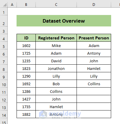
You can see that some persons are missing on the day of taking the vaccine and we want to find out the missing persons. Here we will use the ISERROR, VLOOKUP functions to deal with the missing data. In order to do so, proceed with the following steps.
Steps:
- First of all, create a column and apply the following formula to the selected cell.
=ISERROR(VLOOKUP(C5,$D$5:$D$14,1,0))
Here,
- C5= the data to find
- $D$5:$D$14= Lookup array
Formula Breakdown
The VLOOKUP function considers C5 as the lookup_value and $D$5:$D$14 as lookup array, 1 as col_index_num, and 0 as range lookup.
The ISERROR function returns TRUE as it finds an error or FALSE where it doesn’t find an error. So, when the LOOKUP function doesn’t find a value and makes an error, the ISERROR function returns TRUE, otherwise FALSE.

- Then, use the Fill Handle tool to Autofill the formula for the next cells and you will get the output for the missing data.

- Here, you can also apply Conditional Formatting to highlight the missing data. For this, just select the column> go to Conditional Formatting> select Highlight Cells Rules> select Equal to> select the cell (i.e. E6)> choose Fill Color> click OK.

Note: You can also highlight data manually from the Home tab by changing Text Color or Fill Color.
Read More: How to Filter Missing Data in Excel
2. Using NOT, ISNUMBER, MATCH Functions
For our previous set of data, now we want to show the use of NOT, ISNUMBER and MATCH functions to deal with the missing data. For this, just follow the steps below.
Steps:
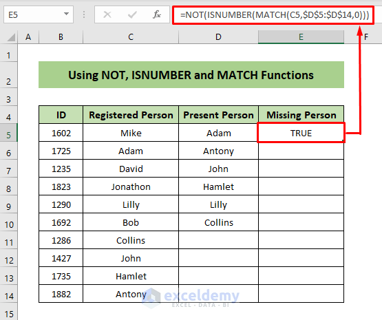
- Firstly, create a new column for the missing data and apply the following formula to the selected cell.
=NOT(ISNUMBER(MATCH(C5,$D$5:$D$14,0)))
Here,
- C5= the data to find
- $D$5:$D$14= Lookup Array
Formula Breakdown
The MATCH function looks up C5 in the $D$5:$D$14 range which is the lookup array.
The cell value of C5 is missing in the lookup array.
The ISNUMBER function gives the output as TRUE or FALSE.
So, ISNUMBER(MATCH(C5,$D$5:$D$14,0)) returns FALSE.
Hence, NOT function turns this FALSE into TRUE.
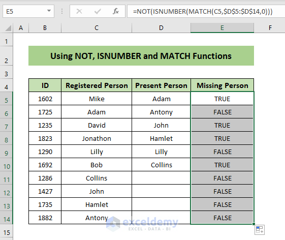
- Then, drag the formula for the next cells to find missing values.
- Then, highlight the missing data with Conditional Formatting like the last step of Method 1.

Read More: How to Fill Missing Values in Excel
3. Extract Missing Data Using IF, ISERROR and VLOOKUP Functions
In the previous two methods, we have just created output with TRUE for missing data and FALSE for existing data. But now, we want to extract the original missing data from the list of the data table. In order to do so, just proceed with the steps below.
Steps:
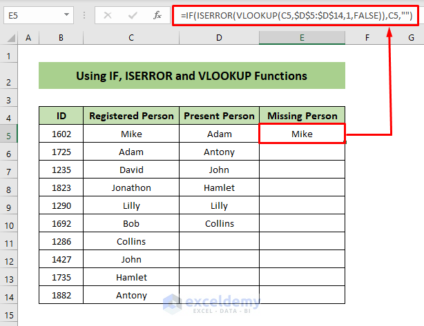
- Firstly, create a new column for the missing person and apply the following formula to the selected cell.
=IF(ISERROR(VLOOKUP(C5,$D$5:$D$14,1,FALSE)),C5,"")
Here,
- C5= the data to find
- $D$5:$D$14= Lookup array
Formula Breakdown
IF function tests the logic and after validation of the logic, it returns C5, otherwise leaves blank (i.e. “ ”)
- Now, just drag the formula down and the column will show only the missing data here.

Read More: How to Find Missing Values in a List in Excel
4. Applying Conditional Formatting
Here, we will now apply Conditional Formatting to find out the missing data for the same dataset. We won’t create a new column here, rather we will just mark the missing data from the existing column. So, let’s start the process like the one below.
Steps:
- First of all, select the two columns (i.e. Registered Person and Present Person). Go to the Home tab> click Conditional Formatting> select New Rule.

- Then, the New Formatting Rule dialogue box will open up. Choose Format only unique or duplicate values from the Select a Rule Type field and select Unique from the Format All field> click Format.

- Now, choose a Fill Color from the Format Cells dialogue box> click OK.

- Here, click OK on the New Formatting Rule box.

- Hence, the main column (i.e. Registered Person) will compare itself to the compared column (i.e. Present Person) and highlight the cells that are missing data.

Read More: How to Compare Two Excel Sheets to Find Missing Data
5. Using IF Function
Let’s say, like the previous dataset, some persons have come to take the vaccine on DAY-1 and some from the DAY-1 along with some new ones have come to take the vaccine on DAY-2. So, some of the persons taken vaccines on DAY-1 are missing on DAY-2.

We want to find the data of the persons from DAY-1 who are missing on DAY-2 by applying the IF function. So, proceed like the steps below.
Steps:
- At first, create a new column for the missing data and apply the following formula to the selected cell.
=IF(B5=C5,"Present","Missing")
Here,
- B5= the data to find from DAY-1
- C5= the data to be compared

- Then, drag the formula for the other cells to get the Missing and the Present data.

Read More: How to Cross Reference in Excel to Find Missing Data
6. Missing Data in Different Sheets
For the previous 5 methods, we have dealt with missing data from the same worksheet. Now, we will deal with data from different worksheets. Here, we have the ID and Name of the persons taking vaccines at DAY-1 on one sheet.

And we have also some information on DAY-2 at another sheet.

We want to find out the person’s names from DAY-2 that are missing on DAY-1. In order to do so, proceed like the steps below.
Steps:
- Firstly, create a new column for the missing persons and apply the following formula.
=IF(ISERROR(VLOOKUP(C5,'DAY-1'!$C$5:$C$14,1,FALSE)),C5,"")
Here,
- C5= the data to find
- $D$5:$D$14= Lookup array

- Then drag the formula down and the cells will show only the missing data.

Read More: How to Find Missing Rows in Excel
Download Practice Workbook
You can download the practice book from the link below.
Conclusion
In this article, I have tried to show you some methods of how to deal with missing data in Excel. I hope this article has shed some light on your way of dealing with missing data in an Excel workbook. If you have better methods, questions, or feedback regarding this article, please don’t forget to share them in the comment box. This will help me enrich my upcoming articles. Have a great day!
Related Articles
<< Go Back To Missing Values in Excel | Data Cleaning in Excel | Learn Excel
Get FREE Advanced Excel Exercises with Solutions!
