How to Find, Count & Fill Missing Values in Excel

Method 1 – Finding Missing Values Using a Combination of IF and COUNTIF Functions

Steps:

Select cell F5.
Enter the formula below:

=IF(COUNTIF($B$5:$B$12,E5),"Available","Not Available")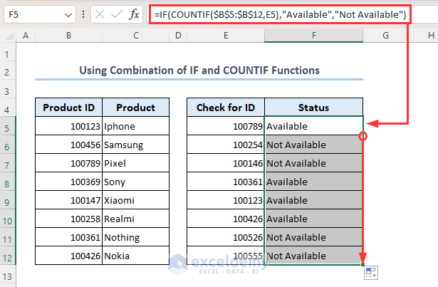

Applying IF and COUNTIF functions to find missing values in Excel

Press Enter.
Drag down the Fill handle icon.

Formula Breakdown

COUNTIF($B$5:$B$12,E5)

This function looks for the value in cell E5 within the range B5:B12. If the value in cell E5 exists within the range B5:B12, then it returns 1. If the value doesn’t exist within the range, then it returns 0.

IF(COUNTIF($B$5:$B$12,E5),”Available”,”Not Available”)

The IF function returns Available if the COUNTIF function returns 1. Otherwise, it returns Not Available.

Method 2 – Finding Missing Values by Combining IF, ISNA, and MATCH Functions

Steps:

Select cell F5.
Enter the formula below:

=IF(ISNA(MATCH(E5,$B$5:$B$12,0)),"Not Available","Available")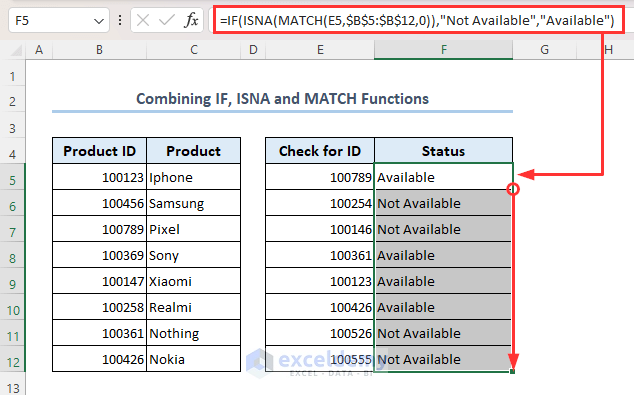

Applying IF, ISNA and MATCH functions to find missing values in Excel

Press Enter.
Drag down using the Fill Handle icon

Formula Breakdown

MATCH(E5,$B$5:$B$12,0)

This function finds the position of the value in cell E5 within the range B5:B12. If the value exists within the range, then the function returns that value’s position. When the value doesn’t exist within the range, the function returns #N/A.

ISNA(MATCH(E5,$B$5:$B$12,0))

If the MATCH function returns the position then the ISNA function returns FALSE. When the MATCH function returns #N/A then the ISNA function returns TRUE.

IF(ISNA(MATCH(E5,$B$5:$B$12,0)),”Not Available”,”Available”)

If the ISNA function returns FALSE, then the IF function returns Available. Other than that, it returns Not Available.

Method 3 – Searching Missing Values by Merging IF, ISNA, and VLOOKUP Functions

Steps:

Select cell F5.
Enter the formula below:

=IF(ISNA(VLOOKUP(E5,$B$5:$B$12,1,FALSE)),"Not Available","Available")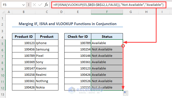

Applying IF, ISNA and VLOOKUP functions to find missing values in Excel

Press Enter.
Uuse the Fill handle to drag down.

Formula Breakdown

VLOOKUP(E5,$B$5:$B$12,1,FALSE)

The VLOOKUP function looks for the corresponding value of cell E5 within the range B5:B12. If the corresponding value exists, then the function returns that value. Otherwise, the function returns #N/A.

ISNA(VLOOKUP(E5,$B$5:$B$12,1,FALSE))

If the VLOOKUP function returns any corresponding value, then the ISNA function returns FALSE. When the VLOOKUP function returns #N/A, then the ISNA function returns TRUE.

IF(ISNA(VLOOKUP(E5,$B$5:$B$12,1,FALSE)),”Not Available”,”Available”)

If the ISNA function returns FALSE, then the IF function returns as Available. If the ISNA function returns TRUE, then the IF function returns Not Available.

Method 4 – Combining IF, ISNUMBER and MATCH Functions

Steps:

Select cell F5.
Enter the formula below:

=IF(ISNUMBER(MATCH(E5,$B$5:$B$12,0)),"Available","Not Available")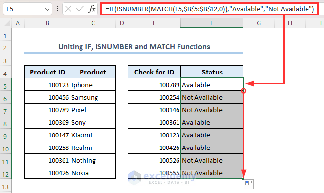

Applying IF, ISNUMBER and MATCH functions to find missing values in Excel

Press Enter.
Drag down using the Fill handle icon.

Formula Breakdown

MATCH(E5,$B$5:$B$12,0)

This function finds the position of the value in cell E5 within the range B5:B12. If the value exists within the range, then the function returns that value’s position. When it doesn’t exist within the range, the function returns #N/A.

ISNUMBER(MATCH(E5,$B$5:$B$12,0))

If the MATCH function returns the position, then the ISNUMBER function returns TRUE. Otherwise, it returns FALSE if the MATCH function returns #N/A.

IF(ISNUMBER(MATCH(E5,$B$5:$B$12,0)),”Available”,”Not Available”)

Finally, for the TRUE statement returned by the ISNUMBER function, the IF function returns Available. And for the FALSE statement, it returns Not Available.

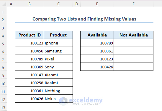
How to Compare Two Lists for Missing Values in Excel

Let’s say you have a range B4:B12 containing several product IDs and another range E5:E8 showing only the available product IDs from the range B4:B12. Now, we want to determine which products from the range B4:B12 are not available.

Dataset representing all products and available products

Steps:

Select cell F5.
Enter the formula below:

=FILTER(B5:B12,COUNTIF(E5:E8,B5:B12)=0)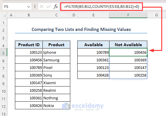

Applying FILTER and COUNTIF functions to find not available products

Press Enter.
This will return all the product IDs from the range B4:B12 that aren’t mentioned in column E.

Formula Breakdown

COUNTIF(E5:E8,B5:B12)

First, the COUNTIF function goes through the range B5:B12 and returns 1 if any value in range B5:B12 exists in range E5:E8. If not, then it returns 0.

FILTER(B5:B12,COUNTIF(E5:E8,B5:B12)=0)

The FILTER function returns those values from range B5:B12, for which the COUNTIF function returns 0.

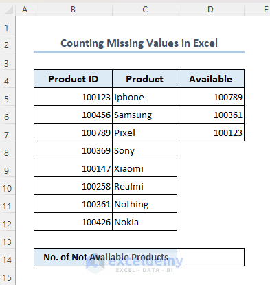
How to Count Missing Values in Excel

Suppose you have a dataset in which range B5:B12 contains some products’ ID numbers, and range D5:D7 shows the available product IDs. We want to calculate the total number of products in range B5:B12 but missing in range D5:D7.

Dataset representing all products and available products of a shop

Steps:

Select cell D14.
Enter the formula below:

=SUMPRODUCT(--(COUNTIF(D5:D7,B5:B12)=0))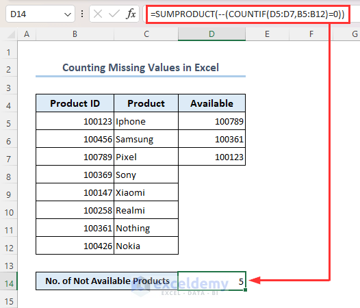

Applying COUNTIF and SUMPRODUCT functions to count missing values in Excel

Press Enter.

Formula Breakdown

COUNTIF(D5:D7,B5:B12)

First, the COUNTIF function goes through the range B5:B12 and returns 1 if any value is found in the range B5:B12 and range E5:E8. If not, then it returns 0.

SUMPRODUCT(–(COUNTIF(D5:D7,B5:B12)=0))

The SUMPRODUCT function will return the sum of the 0 returned by the COUNTIF function.

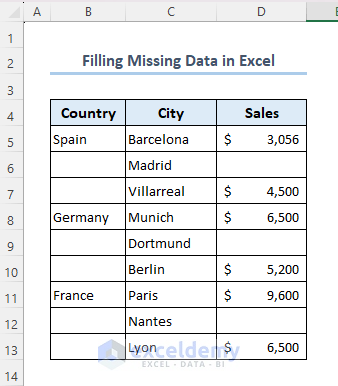
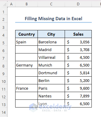
How to Fill Missing Data in Excel

Assume you have a dataset that represents some city’s total sales. However, some cities’ total sales value is missing. So now, we want to fill those missing values with trending values using Excel’s built-in Fill Series feature.

Dataset representing some city’s total sales

Steps:

Select range D5:D7.
Follow these steps: Home >> Editing >> Fill >> Series.

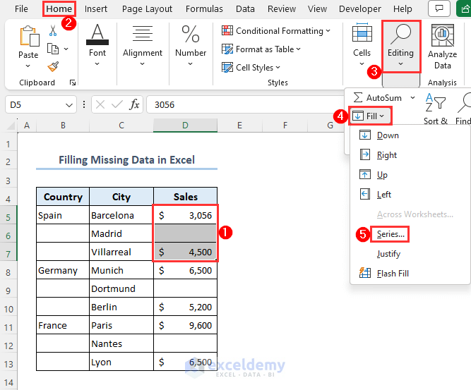
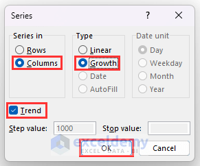
Using fill series feature from the home tab

A dialog box will appear on your screen, as shown below.
Mark Columns, Growth, and Trend.
Click OK.

A dialog box titled “Series” appeared

You will find the result as follows.

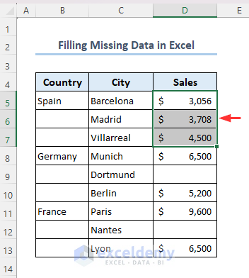
Final output after using the fill series feature

Following a similar procedure for the rest of the cities will return the output as follows.

Completed result after using the fill series feature for rest of the missing values Read More: How to Fill Missing Values in Excel

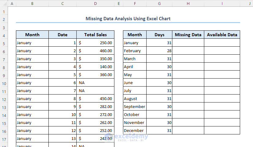
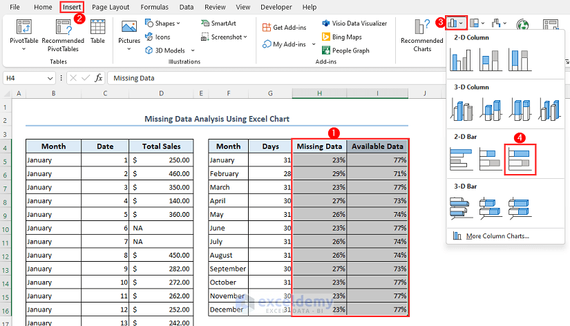
How to Analyze Missing Data Using an Excel Chart

Let’s say we have a dataset that represents a shop’s daily total sales record for 2022. We can see that total sales records are unavailable (NA) for some days. So we consider the total sales values of these days as missing data.

Dataset representing a shop’s daily total sales record for the year 2022

Steps:

Select cell H5.
Enter the formula below:

=COUNTIFS($B$5:$B$369,F5,$D$5:$D$369,"NA")/G5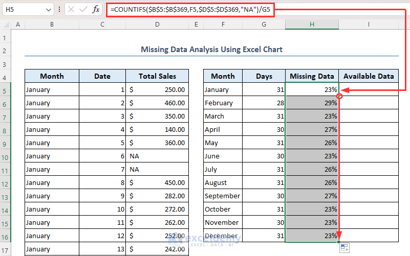

Applying COUNTIF formula to calculate the total number of missing data of a month

Press Enter.
Drag down using the Fill handle
Select cell I5.

Enter the formula below:

=1-H5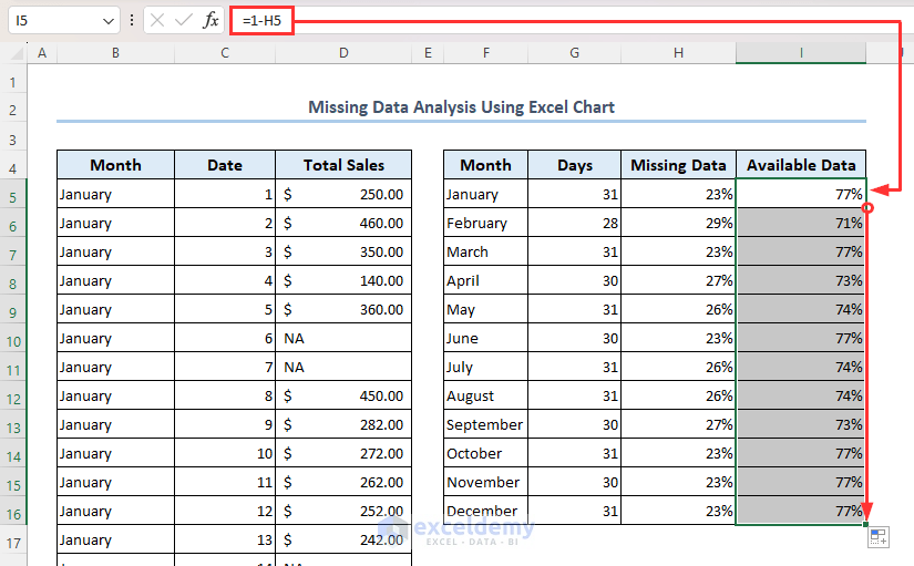

Applying formula to calculate the total number of available data for a month

Press Enter.
Use the Fill handle to drag down.

Select range H4:I16.
Go through these steps: Insert >> Insert Column or Bar Chart >> 100% Stacked Bar.

Using the chart feature

Following this will return you a chart as follows.

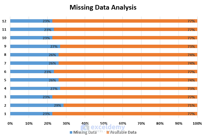
Created chart representing percentage of available and missing data

The chart shows the percentage of missing and available data for each month, with the missing data represented in blue and the available data represented in orange.

Download the Practice Workbook

Missing Values in Excel.xlsx