Dataset Overview
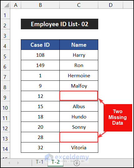
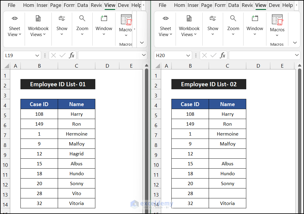
To illustrate the methods, we’ll consider two employee data lists stored in separate sheets: T-1 and T-2.
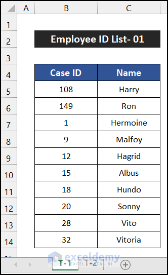
Additionally, there are two blank cells in the data table of sheet T-2, located at cells C9 and C13. Let’s explore seven distinct methods to identify these missing values.
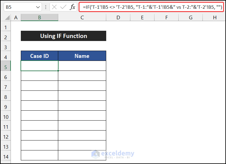
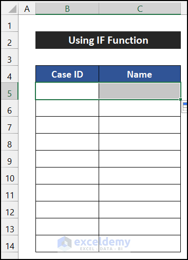
Method 1 – Using the IF Function
- Create a new sheet by clicking the Plus (+) sign in the Sheet Name Bar.
- In cell B5 of the new sheet, enter the following formula:
=IF('T-1'!B5 <> 'T-2'!B5, "T-1:"&'T-1'!B5&" vs T-2:"&'T-2'!B5, "")
- Press Enter.
- Drag the Fill Handle icon to the right to copy the formula up to cell C5.
- Select the range of cells B5:C5 and drag the Fill Handle icon to copy the formula up to cell C14.
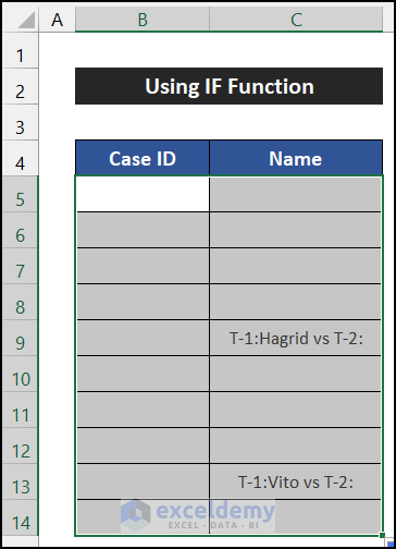
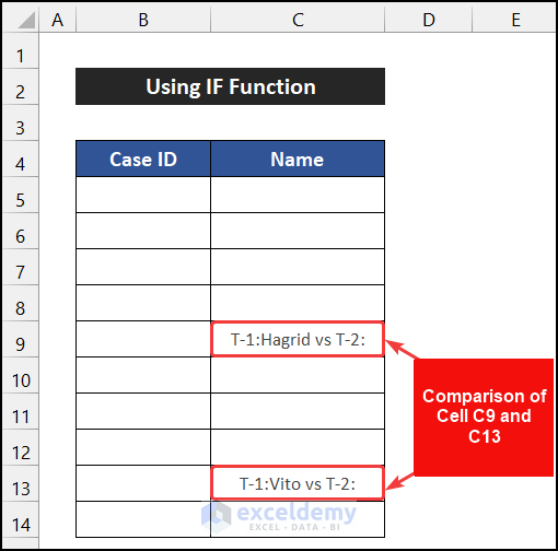
- Observe that cells C9 and C13 display the cell value from sheet T-1 and the missing value from sheet T-2. This confirms that our formula successfully compared the two Excel sheets to find missing data.
Read More: How to Deal with Missing Data in Excel
Method 2 – Applying the VLOOKUP Function
- Select cell D5.
- Enter the following formula in the cell:
=VLOOKUP(B5,'T-2'!$B$4:$C$14,2,FALSE)
- Press Enter.
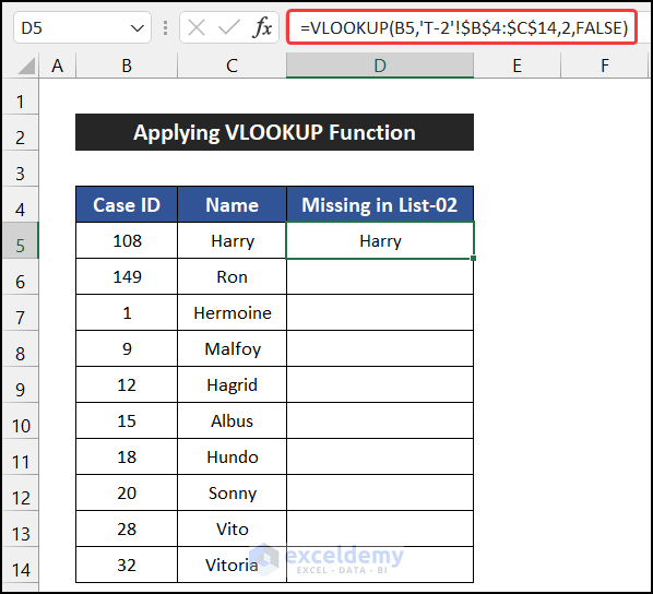
- Double-click the Fill Handle icon to copy the formula up to cell D14.
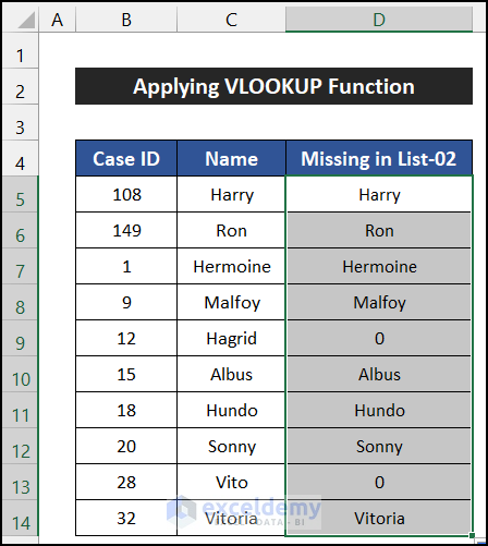
- Note that the formula displays values for all cells except D9 and D13, where it shows Zero (0) for missing values.
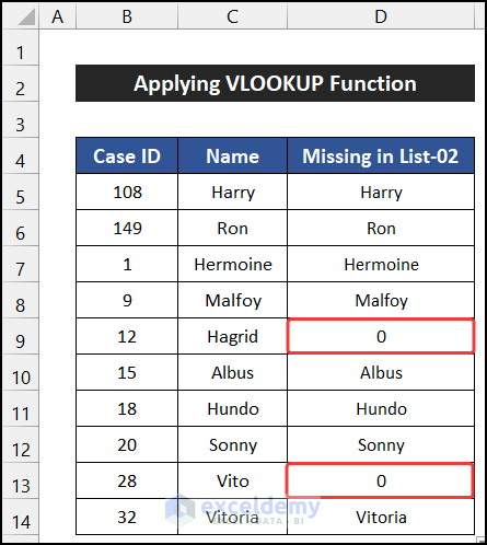
Thus, our formula effectively compared the two Excel sheets to find missing data.
Interpretation of the Result
In the range of cells B5:C14, we have data from sheet T-1. We utilize the VLOOKUP function, which searches for the Case ID from sheet T-1 and retrieves the corresponding value from sheet T-2. Since cells C9 and C13 in sheet T-2 are blank, the formula returns a value of zero (0).
Read More: How to Filter Missing Data in Excel
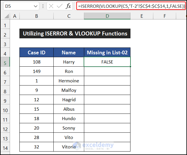
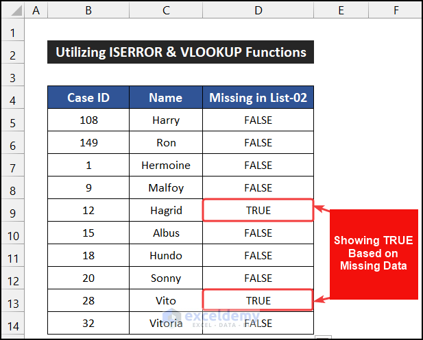
Method 3 – Using the ISERROR and VLOOKUP Functions
- Select cell D5.
- In that cell, enter the following formula:
=ISERROR(VLOOKUP(C5,'T-2'!$C$4:$C$14,1,FALSE))
- Press Enter.
- Double-click the Fill Handle icon to copy the formula up to cell D14.
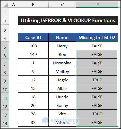
- You’ll observe that cells D9 and D13 return TRUE, while all other cells show FALSE.
Interpretation of the Result
- The data in the range of cells B5:C14 corresponds to sheet T-1.
- The ISERROR function checks the value returned by the VLOOKUP function.
- When the value matches, ISERROR returns FALSE.
- If there’s a blank cell, the function returns TRUE.
Breakdown of the Formula
We are breaking down the formula for cell D9.
- VLOOKUP(C9,’T-2′!$C$4:$C$14,1,FALSE): This function checks for an exact match of the cell value C5 in sheet T-2. Since the value isn’t available in sheet T-2 for the corresponding match, the function returns #N/A.
- ISERROR(VLOOKUP(C9,’T-2′!$C$4:$C$14,1,FALSE)): The ISERROR function verifies whether the result of the VLOOKUP function is an error. In this case, the result isn’t an error, so it returns TRUE.
Read More: How to Find Missing Values in Excel
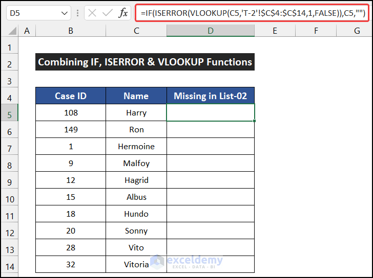
Method 4 – Combing the IF, ISERROR and VLOOKUP Functions
- Select cell D5.
- In that cell, enter the following formula:
=IF(ISERROR(VLOOKUP(C5,'T-2'!$C$4:$C$14,1,FALSE)),C5,"")
- Press Enter.
- Double-click the Fill Handle icon to copy the formula up to cell D14.
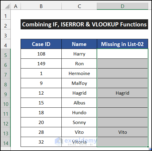
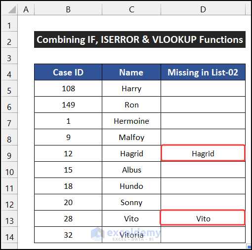
- You’ll notice that cells C9 and C13 from sheet T-2 display the missing values, which correspond to the values in the corresponding cells.
Breakdown of the Formula
We are breaking down the formula for cell D9.
- VLOOKUP(C9,’T-2′!$C$4:$C$14,1,FALSE): This function checks for an exact match of the cell value C5 in sheet T-2. Since the value isn’t available in sheet T-2 for the corresponding match, the function returns #N/A.
- ISERROR(VLOOKUP(C9,’T-2′!$C$4:$C$14,1,FALSE)): The ISERROR function verifies whether the result of the VLOOKUP function is an error. In this case, the result isn’t an error, so it returns TRUE.
- IF(ISERROR(VLOOKUP(C9,’T-2′!$C$4:$C$14,1,FALSE)),C9,””): The IF function checks the result of the ISERROR function. If the logic is true (i.e., there’s an error), it shows the value of C9. Otherwise, it returns blank. In this cell, the function returns the value of cell C9, which is Hagrid.
Method 5 – Using the NOT, ISNUMBER and MATCH Functions
- Select cell D5.
- In that cell, enter the following formula:
=NOT(ISNUMBER(MATCH(C5,'T-2'!$C$4:$C$14,0)))
- Press Enter.
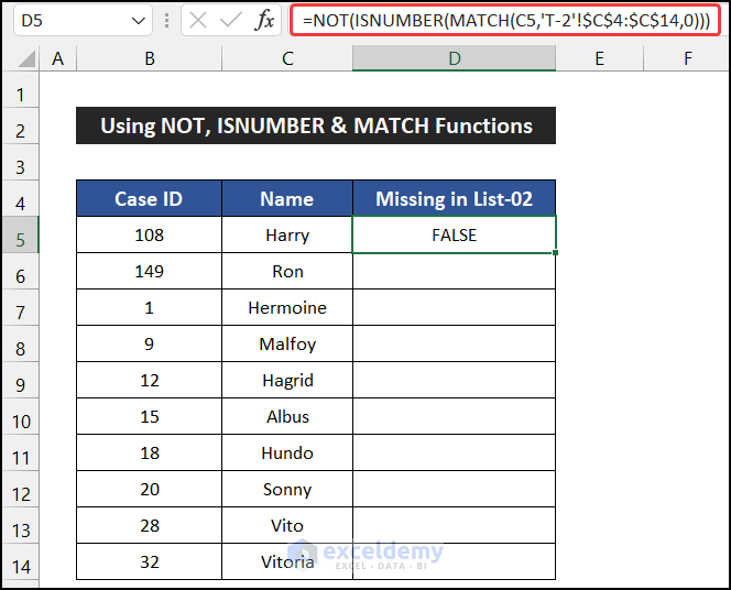
- Double-click the Fill Handle icon to copy the formula up to cell D14.
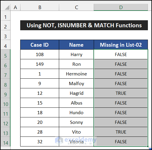
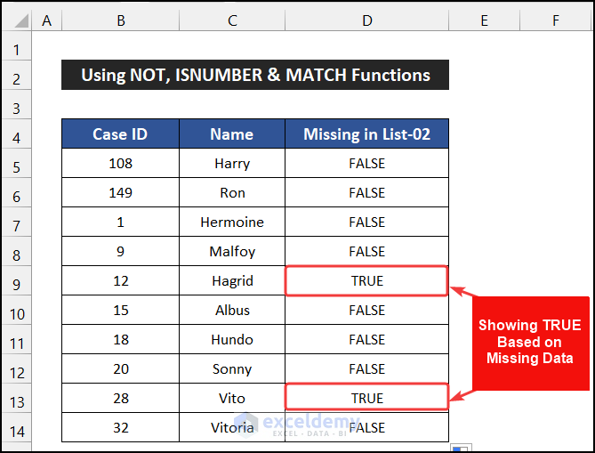
- You’ll notice that cells D9 and D13 return TRUE, while all other cells show FALSE.
Interpretation of the Result
- The data in the range of cells B5:C14 corresponds to sheet T-1.
- The combined formula of NOT, ISNUMBER, and MATCH functions returns FALSE when the cells of sheet T-2 contain data.
- However, when there is a blank cell, the formula returns TRUE.
Breakdown of the Formula
We are breaking down the formula for cell D9.
- MATCH(C9,’T-2′!$C$4:$C$14,0): This function finds the match of the value in cell C5 within the datasheet T-2. Since the value isn’t available in sheet T-2, the function returns #N/A.
- ISNUMBER(MATCH(C9,’T-2′!$C$4:$C$14,0)): The ISNUMBER function checks whether the result of the match function is a number. For this cell, the result is not a number, so it returns FALSE.
- NOT(ISNUMBER(MATCH(C9,’T-2′!$C$4:$C$14,0))): The NOT function toggles the result of the ISNUMBER function. In this case, the formula returns TRUE.
Read More: How to Cross Reference in Excel to Find Missing Data
Method 6 – Using the “Arrange All” Command from the View Tab
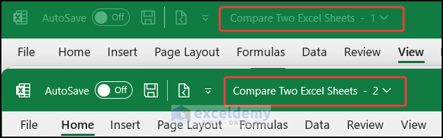
- Open your Excel workbook.
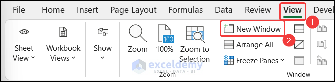
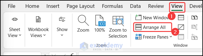
- Go to the View tab.
- Click on the New Window command in the Window group. This will create a copy of your current workbook.
- A new window with the copied workbook will appear.
- Return to the View tab and select the Arrange All command.
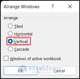
- In the Arrange Window dialog box, choose the Vertical option.
- Click OK.
- You’ll see both workbooks side by side, allowing you to manually compare the sheets and identify missing data.
Read More: How to Fill Missing Values in Excel
Method 7 – Embedding VBA Code
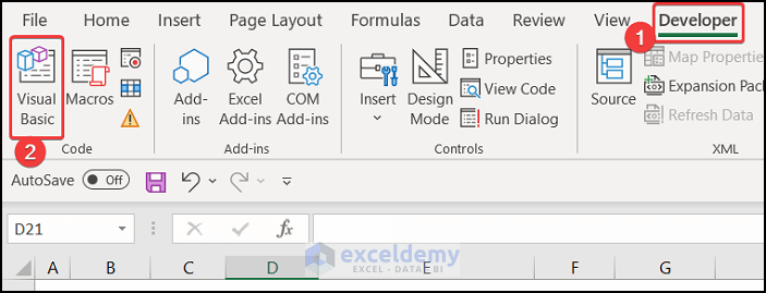
- Go to the Developer tab.
- Click on Visual Basic or press Alt+F11 to open the Visual Basic Editor.
- In the editor, click the Insert tab and choose Module.

- Enter the following VBA code in the empty editor:

Sub Compare_Two_Sheets()
Dim Rng_Cell As Range
For Each Rng_Cell In Worksheets("T-1").Range("B4:C14")
    If Not Rng_Cell = Worksheets("T-2").Cells(Rng_Cell.Row, Rng_Cell.Column) Then
        Rng_Cell.Interior.Color = vbYellow
    End If
Next Rng_Cell
End Sub- Save the code by pressing Ctrl+S.
- Close the editor.
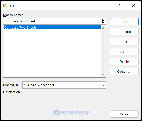
- Back in Excel, go to the Developer tab and click on Macros.

- Select Compare_Two_Sheets and click Run to execute the code.
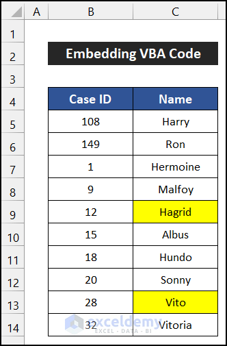
- The cells with missing values from sheet T-2 will be highlighted in yellow.
Download Practice Workbook
You can download the practice workbook from here:
Related Articles
- How to Find Missing Rows in Excel
- Count Missing Values in Excel
- How to Remove Missing Values in Excel
<< Go Back To Missing Values in Excel | Data Cleaning in Excel | Learn Excel
Get FREE Advanced Excel Exercises with Solutions!
